�
1
Introduction to Compressed
Sensing
Mark A. Davenport
Stanford University, Department of Statistics
Marco F. Duarte
Duke University, Department of Computer Science
Yonina C. Eldar
Technion, Israel Institute of Technology, Department of Electrical Engineering
Stanford University, Department of Electrical Engineering (Visiting)
Gitta Kutyniok
University of Osnabrueck, Institute for Mathematics
In recent years, compressed sensing (CS) has attracted considerable attention
in areas of applied mathematics, computer science, and electrical engineering
by suggesting that it may be possible to surpass the traditional limits of sam-
pling theory. CS builds upon the fundamental fact that we can represent many
signals using only a few non-zero coefficients in a suitable basis or dictionary.
Nonlinear optimization can then enable recovery of such signals from very few
measurements. In this chapter, we provide an up-to-date review of the basic
theory underlying CS. After a brief historical overview, we begin with a dis-
cussion of sparsity and other low-dimensional signal models. We then treat the
central question of how to accurately recover a high-dimensional signal from a
small set of measurements and provide performance guarantees for a variety of
sparse recovery algorithms. We conclude with a discussion of some extensions
of the sparse recovery framework. In subsequent chapters of the book, we will
see how the fundamentals presented in this chapter are extended in many excit-
ing directions, including new models for describing structure in both analog and
discrete-time signals, new sensing design techniques, more advanced recovery
results, and emerging applications.
1.1
Introduction
We are in the midst of a digital revolution that is driving the development and
deployment of new kinds of sensing systems with ever-increasing fidelity and
resolution. The theoretical foundation of this revolution is the pioneering work
of Kotelnikov, Nyquist, Shannon, and Whittaker on sampling continuous-time
band-limited signals [162, 195, 209, 247]. Their results demonstrate that signals,
1
2
Chapter 1.
Introduction to Compressed Sensing
images, videos, and other data can be exactly recovered from a set of uniformly
spaced samples taken at the so-called Nyquist rate of twice the highest frequency
present in the signal of interest. Capitalizing on this discovery, much of signal
processing has moved from the analog to the digital domain and ridden the wave
of Moore’s law. Digitization has enabled the creation of sensing and processing
systems that are more robust, flexible, cheaper and, consequently, more widely
used than their analog counterparts.
As a result of this success, the amount of data generated by sensing systems
has grown from a trickle to a torrent. Unfortunately, in many important and
emerging applications, the resulting Nyquist rate is so high that we end up with
far too many samples. Alternatively, it may simply be too costly, or even physi-
cally impossible, to build devices capable of acquiring samples at the necessary
rate [146, 241]. Thus, despite extraordinary advances in computational power, the
acquisition and processing of signals in application areas such as imaging, video,
medical imaging, remote surveillance, spectroscopy, and genomic data analysis
continues to pose a tremendous challenge.
To address the logistical and computational challenges involved in dealing
with such high-dimensional data, we often depend on compression, which aims
at finding the most concise representation of a signal that is able to achieve
a target level of acceptable distortion. One of the most popular techniques for
signal compression is known as transform coding, and typically relies on finding
a basis or frame that provides sparse or compressible representations for signals
in a class of interest [31, 77, 106]. By a sparse representation, we mean that for
a signal of length n, we can represent it with k n nonzero coefficients; by a
compressible representation, we mean that the signal is well-approximated by
a signal with only k nonzero coefficients. Both sparse and compressible signals
can be represented with high fidelity by preserving only the values and locations
of the largest coefficients of the signal. This process is called sparse approxima-
tion, and forms the foundation of transform coding schemes that exploit signal
sparsity and compressibility, including the JPEG, JPEG2000, MPEG, and MP3
standards.
Leveraging the concept of transform coding, compressed sensing (CS) has
emerged as a new framework for signal acquisition and sensor design. CS enables
a potentially large reduction in the sampling and computation costs for sensing
signals that have a sparse or compressible representation. While the Nyquist-
Shannon sampling theorem states that a certain minimum number of samples
is required in order to perfectly capture an arbitrary bandlimited signal, when
the signal is sparse in a known basis we can vastly reduce the number of mea-
surements that need to be stored. Consequently, when sensing sparse signals we
might be able to do better than suggested by classical results. This is the fun-
damental idea behind CS: rather than first sampling at a high rate and then
compressing the sampled data, we would like to find ways to directly sense the
data in a compressed form — i.e., at a lower sampling rate. The field of CS grew
out of the work of Cand`es, Romberg, and Tao and of Donoho, who showed that
�
Introduction to Compressed Sensing
3
a finite-dimensional signal having a sparse or compressible representation can
be recovered from a small set of linear, nonadaptive measurements [3, 33, 40–
42, 44, 82]. The design of these measurement schemes and their extensions to
practical data models and acquisition systems are central challenges in the field
of CS.
While this idea has only recently gained significant attraction in the signal
processing community, there have been hints in this direction dating back as far
as the eighteenth century. In 1795, Prony proposed an algorithm for the estima-
tion of the parameters associated with a small number of complex exponentials
sampled in the presence of noise [201]. The next theoretical leap came in the early
1900’s, when Carath´eodory showed that a positive linear combination of any k
sinusoids is uniquely determined by its value at t = 0 and at any other 2k points
in time [46, 47]. This represents far fewer samples than the number of Nyquist-
rate samples when k is small and the range of possible frequencies is large. In the
1990’s, this work was generalized by George, Gorodnitsky, and Rao, who studied
sparsity in biomagnetic imaging and other contexts [134–136, 202]. Simultane-
ously, Bresler, Feng, and Venkataramani proposed a sampling scheme for acquir-
ing certain classes of signals consisting of k components with nonzero bandwidth
(as opposed to pure sinusoids) under restrictions on the possible spectral sup-
ports, although exact recovery was not guaranteed in general [29, 117, 118, 237].
In the early 2000’s Blu, Marziliano, and Vetterli developed sampling methods
for certain classes of parametric signals that are governed by only k param-
eters, showing that these signals can be sampled and recovered from just 2k
samples [239].
A related problem focuses on recovery of a signal from partial observation of
its Fourier transform. Beurling proposed a method for extrapolating these obser-
vations to determine the entire Fourier transform [22]. One can show that if the
signal consists of a finite number of impulses, then Beurling’s approach will cor-
rectly recover the entire Fourier transform (of this non-bandlimited signal) from
any sufficiently large piece of its Fourier transform. His approach — to find the
signal with smallest 1 norm among all signals agreeing with the acquired Fourier
measurements — bears a remarkable resemblance to some of the algorithms used
in CS.
More recently, Cand`es, Romberg, Tao [33, 40–42, 44], and Donoho [82] showed
that a signal having a sparse representation can be recovered exactly from a
small set of linear, nonadaptive measurements. This result suggests that it may
be possible to sense sparse signals by taking far fewer measurements, hence the
name compressed sensing. Note, however, that CS differs from classical sampling
in three important respects. First, sampling theory typically considers infinite
length, continuous-time signals. In contrast, CS is a mathematical theory focused
on measuring finite-dimensional vectors in Rn. Second, rather than sampling the
signal at specific points in time, CS systems typically acquire measurements in
the form of inner products between the signal and more general test functions.
This is in fact in the spirit of modern sampling methods which similarly acquire
�
4
Chapter 1.
Introduction to Compressed Sensing
signals by more general linear measurements [113, 230]. We will see throughout
this book that randomness often plays a key role in the design of these test
functions. Thirdly, the two frameworks differ in the manner in which they deal
with signal recovery, i.e., the problem of recovering the original signal from the
compressive measurements. In the Nyquist-Shannon framework, signal recovery
is achieved through sinc interpolation — a linear process that requires little
computation and has a simple interpretation. In CS, however, signal recovery is
typically achieved using highly nonlinear methods.1 See Section 1.6 as well as
the survey in [226] for an overview of these techniques.
CS has already had notable impact on several applications. One example is
medical imaging [178–180, 227], where it has enabled speedups by a factor of
seven in pediatric MRI while preserving diagnostic quality [236]. Moreover, the
broad applicability of this framework has inspired research that extends the
CS framework by proposing practical implementations for numerous applica-
tions, including sub-Nyquist sampling systems [125, 126, 186–188, 219, 224, 225,
228], compressive imaging architectures [99, 184, 205], and compressive sensor
networks [7, 72, 141].
The aim of this book is to provide an up-to-date review of some of the impor-
tant results in CS. Many of the results and ideas in the various chapters rely
on the fundamental concepts of CS. Since the focus of the remaining chapters
is on more recent advances, we concentrate here on many of the basic results in
CS that will serve as background material to the rest of the book. Our goal in
this chapter is to provide an overview of the field and highlight some of the key
technical results, which are then more fully explored in subsequent chapters. We
begin with a brief review of the relevant mathematical tools, and then survey
many of the low-dimensional models commonly used in CS, with an emphasis
on sparsity and the union of subspaces models. We next focus attention on the
theory and algorithms for sparse recovery in finite dimensions. To facilitate our
goal of providing both an elementary introduction as well as a comprehensive
overview of many of the results in CS, we provide proofs of some of the more
technical lemmas and theorems in the Appendix.
1.2
Review of Vector Spaces
For much of its history, signal processing has focused on signals produced by
physical systems. Many natural and man-made systems can be modeled as linear.
Thus, it is natural to consider signal models that complement this kind of linear
structure. This notion has been incorporated into modern signal processing by
modeling signals as vectors living in an appropriate vector space. This captures
1 It is also worth noting that it has recently been shown that nonlinear methods can be used in
the context of traditional sampling as well, when the sampling mechanism is nonlinear [105].
�
Introduction to Compressed Sensing
5
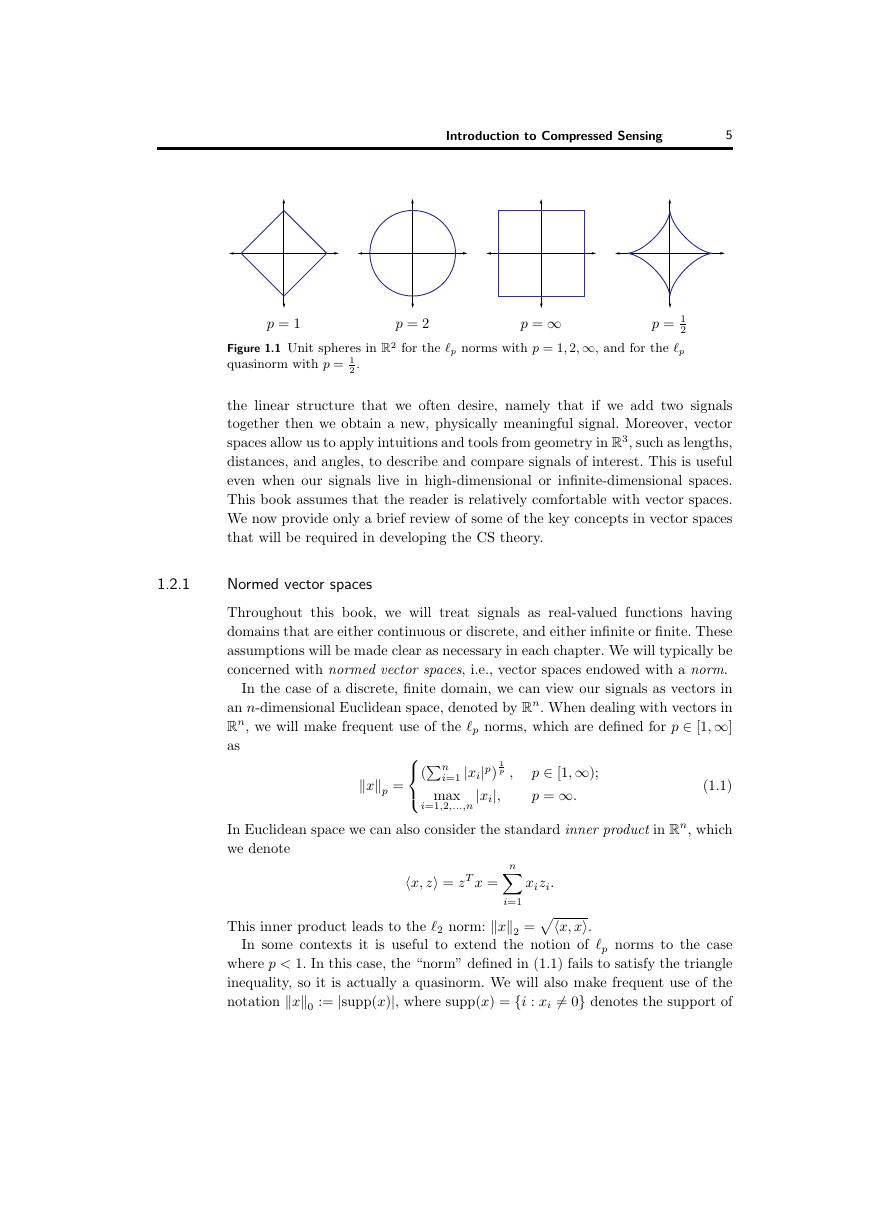
p = 1
p = 1
2
Figure 1.1 Unit spheres in R2 for the p norms with p = 1, 2,∞, and for the p
quasinorm with p = 1
2 .
p = 2
p = ∞
the linear structure that we often desire, namely that if we add two signals
together then we obtain a new, physically meaningful signal. Moreover, vector
spaces allow us to apply intuitions and tools from geometry in R3, such as lengths,
distances, and angles, to describe and compare signals of interest. This is useful
even when our signals live in high-dimensional or infinite-dimensional spaces.
This book assumes that the reader is relatively comfortable with vector spaces.
We now provide only a brief review of some of the key concepts in vector spaces
that will be required in developing the CS theory.
1.2.1
Normed vector spaces
Throughout this book, we will treat signals as real-valued functions having
domains that are either continuous or discrete, and either infinite or finite. These
assumptions will be made clear as necessary in each chapter. We will typically be
concerned with normed vector spaces, i.e., vector spaces endowed with a norm.
In the case of a discrete, finite domain, we can view our signals as vectors in
an n-dimensional Euclidean space, denoted by Rn. When dealing with vectors in
Rn, we will make frequent use of the p norms, which are defined for p ∈ [1,∞]
as
xp =
p ∈ [1,∞);
p = ∞.
(1.1)
In Euclidean space we can also consider the standard inner product in Rn, which
we denote
(n
i=1 |xi|p)
1
p ,
|xi|,
max
i=1,2,...,n
n
This inner product leads to the 2 norm: x2 =x, x.
xizi.
i=1
x, z = zT x =
In some contexts it is useful to extend the notion of p norms to the case
where p < 1. In this case, the “norm” defined in (1.1) fails to satisfy the triangle
inequality, so it is actually a quasinorm. We will also make frequent use of the
notation x0 := |supp(x)|, where supp(x) = {i : xi = 0} denotes the support of
�
6
Chapter 1.
Introduction to Compressed Sensing
p = 1
p = 2
p = ∞
p = 1
2
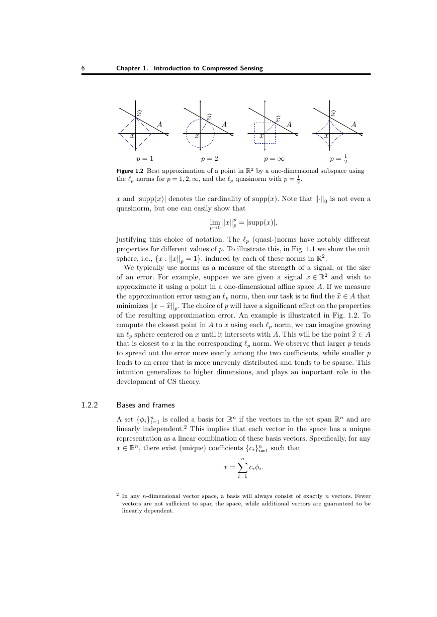
Figure 1.2 Best approximation of a point in R2 by a one-dimensional subspace using
the p norms for p = 1, 2,∞, and the p quasinorm with p = 1
2 .
x and |supp(x)| denotes the cardinality of supp(x). Note that ·0 is not even a
quasinorm, but one can easily show that
xp
p = |supp(x)|,
lim
p→0
justifying this choice of notation. The p (quasi-)norms have notably different
properties for different values of p. To illustrate this, in Fig. 1.1 we show the unit
sphere, i.e., {x : xp = 1}, induced by each of these norms in R2.
We typically use norms as a measure of the strength of a signal, or the size
of an error. For example, suppose we are given a signal x ∈ R2 and wish to
the approximation error using an p norm, then our task is to find thex ∈ A that
approximate it using a point in a one-dimensional affine space A. If we measure
minimizes x −xp. The choice of p will have a significant effect on the properties
an p sphere centered on x until it intersects with A. This will be the pointx ∈ A
of the resulting approximation error. An example is illustrated in Fig. 1.2. To
compute the closest point in A to x using each p norm, we can imagine growing
that is closest to x in the corresponding p norm. We observe that larger p tends
to spread out the error more evenly among the two coefficients, while smaller p
leads to an error that is more unevenly distributed and tends to be sparse. This
intuition generalizes to higher dimensions, and plays an important role in the
development of CS theory.
1.2.2
Bases and frames
A set {φi}n
i=1 is called a basis for Rn if the vectors in the set span Rn and are
linearly independent.2 This implies that each vector in the space has a unique
representation as a linear combination of these basis vectors. Specifically, for any
x ∈ Rn, there exist (unique) coefficients {ci}n
i=1 such that
n
x =
ciφi.
i=1
2 In any n-dimensional vector space, a basis will always consist of exactly n vectors. Fewer
vectors are not sufficient to span the space, while additional vectors are guaranteed to be
linearly dependent.
xAxAxxxAxxAx�
Introduction to Compressed Sensing
7
Note that if we let Φ denote the n × n matrix with columns given by φi and let
c denote the length-n vector with entries ci, then we can represent this relation
more compactly as
x = Φc.
An important special case of a basis is an orthonormal basis, defined as a set
of vectors {φi}n
i=1 satisfying
φi, φj =
1,
0,
i = j;
i = j.
An orthonormal basis has the advantage that the coefficients c can be easily
calculated as
or
ci = x, φi,
c = ΦT x
in matrix notation. This can easily be verified since the orthonormality of the
columns of Φ means that ΦT Φ = I, where I denotes the n × n identity matrix.
It is often useful to generalize the concept of a basis to allow for sets of possibly
linearly dependent vectors, resulting in what is known as a frame [48, 55, 65,
163, 164, 182]. More formally, a frame is a set of vectors {φi}n
i=1 in Rd, d < n
corresponding to a matrix Φ ∈ Rd×n, such that for all vectors x ∈ Rd,
2 ≤ΦT x2
Ax2
2 ≤ B x2
2
with 0 < A ≤ B < ∞. Note that the condition A > 0 implies that the rows of Φ
must be linearly independent. When A is chosen as the largest possible value and
B as the smallest for these inequalities to hold, then we call them the (optimal)
frame bounds. If A and B can be chosen as A = B, then the frame is called
A-tight, and if A = B = 1, then Φ is a Parseval frame. A frame is called equal-
norm, if there exists some λ > 0 such that φi2 = λ for all i = 1, . . . , n, and it
is unit-norm if λ = 1. Note also that while the concept of a frame is very general
and can be defined in infinite-dimensional spaces, in the case where Φ is a d × n
matrix A and B simply correspond to the smallest and largest eigenvalues of
ΦΦT , respectively.
Frames can provide richer representations of data due to their redundancy [26]:
for a given signal x, there exist infinitely many coefficient vectors c such that
x = Φc. In order to obtain a set of feasible coefficients we exploit the dual frame
Φ. Specifically, any frame satisfying
ΦΦT =ΦΦT = I
is called an (alternate) dual frame. The particular choice ˜Φ = (ΦΦT )−1Φ is
referred to as the canonical dual frame. It is also known as the Moore-Penrose
�




 2023年江西萍乡中考道德与法治真题及答案.doc
 2012年重庆南川中考生物真题及答案.doc
 2013年江西师范大学地理学综合及文艺理论基础考研真题.doc
 2020年四川甘孜小升初语文真题及答案I卷.doc
 2020年注册岩土工程师专业基础考试真题及答案.doc
 2023-2024学年福建省厦门市九年级上学期数学月考试题及答案.doc
 2021-2022学年辽宁省沈阳市大东区九年级上学期语文期末试题及答案.doc
 2022-2023学年北京东城区初三第一学期物理期末试卷及答案.doc
 2018上半年江西教师资格初中地理学科知识与教学能力真题及答案.doc
 2012年河北国家公务员申论考试真题及答案-省级.doc
 2020-2021学年江苏省扬州市江都区邵樊片九年级上学期数学第一次质量检测试题及答案.doc
 2022下半年黑龙江教师资格证中学综合素质真题及答案.doc