IEEE TRANSACTIONS ON PATTERN ANALYSIS AND MACHINE INTELLIGENCE, VOL. 35, NO. 6,
JUNE 2013
1397
Guided Image Filtering
Kaiming He, Member, IEEE, Jian Sun, Member, IEEE, and Xiaoou Tang, Fellow, IEEE
Abstract—In this paper, we propose a novel explicit image filter called guided filter. Derived from a local linear model, the guided filter
computes the filtering output by considering the content of a guidance image, which can be the input image itself or another different
image. The guided filter can be used as an edge-preserving smoothing operator like the popular bilateral filter [1], but it has better
behaviors near edges. The guided filter is also a more generic concept beyond smoothing: It can transfer the structures of the guidance
image to the filtering output, enabling new filtering applications like dehazing and guided feathering. Moreover, the guided filter
naturally has a fast and nonapproximate linear time algorithm, regardless of the kernel size and the intensity range. Currently, it is one
of the fastest edge-preserving filters. Experiments show that the guided filter is both effective and efficient in a great variety of
computer vision and computer graphics applications, including edge-aware smoothing, detail enhancement, HDR compression, image
matting/feathering, dehazing, joint upsampling, etc.
Index Terms—Edge-preserving filtering, bilateral filter, linear time filtering
Ç
1 INTRODUCTION
MOST applications in computer vision and computer
graphics involve image filtering to suppress and/or
extract content in images. Simple linear translation-invariant
(LTI)
filters with explicit kernels, such as the mean,
Gaussian, Laplacian, and Sobel filters [2], have been widely
used in image restoration, blurring/sharpening, edge
detection, feature extraction, etc. Alternatively, LTI filters
can be implicitly performed by solving a Poisson Equation
as in high dynamic range (HDR) compression [3], image
stitching [4],
image matting [5], and gradient domain
manipulation [6]. The filtering kernels are implicitly defined
by the inverse of a homogenous Laplacian matrix.
The LTI filtering kernels are spatially invariant and
independent of image content. But usually one may want
to consider additional information from a given guidance
image. The pioneer work of anisotropic diffusion [7] uses the
gradients of the filtering image itself to guide a diffusion
process, avoiding smoothing edges. The weighted least
squares (WLS) filter [8] utilizes the filtering input (instead
of intermediate results, as in [7]) as the guidance, and
optimizes a quadratic function, which is equivalent to
anisotropic diffusion with a nontrivial steady state. The
guidance image can also be another image besides the
filtering input
in
colorization [9] the chrominance channels should not bleed
across luminance edges; in image matting [10] the alpha
matte should capture the thin structures in a composite
image; in haze removal [11] the depth layer should be
in many applications. For example,
. K. He and J. Sun are with the Visual Computing Group, Microsoft
Research Asia, Microsoft Building 2, #5 Dan Leng Street, Hai Dian
District, Beijing 100080, China. E-mail: {kahe, jiansun}@microsoft.com.
. X. Tang is with the Department of Information Engineering, Chinese
University of Hong Kong, 809 SHB, Shatin, N.T., Hong Kong.
E-mail: xtang@ie.cuhk.edu.hk.
Manuscript received 13 June 2012; revised 6 Sept. 2012; accepted 16 Sept.
2012; published online 1 Oct. 2012.
Recommended for acceptance by J. Jia.
For information on obtaining reprints of this article, please send e-mail to:
tpami@computer.org, and reference IEEECS Log Number
TPAMI-2012-06-0447.
Digital Object Identifier no. 10.1109/TPAMI.2012.213.
consistent with the scene. In these cases, we regard the
chrominance/alpha/depth layers as the image to be
filtered, and the luminance/composite/scene as the gui-
dance image, respectively. The filtering process in [9], [10],
and [11]
is achieved by optimizing a quadratic cost
function weighted by the guidance image. The solution is
given by solving a large sparse matrix which solely
depends on the guide. This inhomogeneous matrix im-
plicitly defines a translation-variant filtering kernel. While
these optimization-based approaches [8], [9], [10], [11] often
yield state-of-the-art quality, it comes with the price of
expensive computational time.
Another way to take advantage of the guidance image is
to explicitly build it into the filter kernels. The bilateral
filter, independently proposed in [12], [13], and [1] and
later generalized in [14], is perhaps the most popular one
of such explicit filters. Its output at a pixel is a weighted
average of the nearby pixels, where the weights depend on
the intensity/color similarities in the guidance image. The
guidance image can be the filter input itself [1] or another
image [14]. The bilateral filter can smooth small fluctua-
tions and while preserving edges. Though this filter is
effective in many situations, it may have unwanted gradient
reversal artifacts [15], [16], [8] near edges (discussed in
Section 3.4). The fast implementation of the bilateral filter
is also a challenging problem. Recent techniques [17], [18],
[19], [20], [21] rely on quantization methods to accelerate
but may sacrifice accuracy.
In this paper, we propose a novel explicit image filter
called guided filter. The filtering output is locally a linear
transform of the guidance image. On one hand, the guided
filter has good edge-preserving smoothing properties like the
bilateral filter, but it does not suffer from the gradient
reversal artifacts. On the other hand, the guided filter can be
used beyond smoothing: With the help of the guidance
image, it can make the filtering output more structured and
less smoothed than the input. We demonstrate that the
guided filter performs very well
in a great variety of
applications,
including image smoothing/enhancement,
HDR compression, flash/no-flash imaging, matting/feath-
ering, dehazing, and joint upsampling. Moreover, the guided
0162-8828/13/$31.00 ß 2013 IEEE
Published by the IEEE Computer Society
�
1398
IEEE TRANSACTIONS ON PATTERN ANALYSIS AND MACHINE INTELLIGENCE, VOL. 35, NO. 6,
JUNE 2013
filter naturally has an OðNÞ time (in the number of pixels N)1
nonapproximate algorithm for both gray-scale and high-
dimensional images, regardless of the kernel size and the
intensity range. Typically, our CPU implementation achieves
40 ms per mega-pixel performing gray-scale filtering: To the
best of our knowledge, this is one of the fastest edge-
preserving filters.
A preliminary version of this paper was published in
ECCV ’10 [22]. It is worth mentioning that the guided filter
has witnessed a series of new applications since then. The
guided filter enables a high-quality real-time OðNÞ stereo
matching algorithm [23]. A similar stereo method is
proposed independently in [24]. The guided filter has also
been applied in optical flow estimation [23], interactive
image segmentation [23], saliency detection [25], and
illumination rendering [26]. We believe that the guided
filter has great potential in computer vision and graphics,
given its simplicity, efficiency, and high-quality. We have
provided a public code to facilitate future studies [27].
2 RELATED WORK
We review edge-preserving filtering techniques in this
section. We categorize them as explicit/implicit weighted-
average filters and nonaverage ones.
2.1 Explicit Weighted-Average Filters
The bilateral
filter [1] is perhaps the simplest and most
intuitive one among explicit weighted-average filters. It
computes the filtering output at each pixel as the average of
neighboring pixels, weighted by the Gaussian of both
spatial and intensity distance. The bilateral filter smooths
the image while preserving edges. It has been widely used
in noise reduction [28], HDR compression [15], multiscale
detail decomposition [29], and image abstraction [30]. It is
generalized to the joint bilateral filter in [14], where the
weights are computed from another guidance image rather
than the filtering input. The joint bilateral
filter is
particularly favored when the image to be filtered is not
reliable to provide edge information, e.g., when it is very
noisy or is an intermediate result, such as in flash/no-flash
denoising [14], image upsamling [31], image deconvolution
[32], stereo matching [33], etc.
The bilateral filter has limitations despite its popularity. It
has been noticed in [15], [16], and [8] that the bilateral filter
may suffer from “gradient reversal” artifacts. The reason is
that when a pixel (often on an edge) has few similar pixels
around it, the Gaussian weighted average is unstable. In this
case, the results may exhibit unwanted profiles around
edges, usually observed in detail enhancement or HDR
compression.
Another issue concerning the bilateral filter is the
efficiency. A brute-force implementation is OðNr2Þ time with
kernel radius r. Durand and Dorsey [15] propose a piece-wise
linear model and enable FFT-based filtering. Paris and
Durand [17] formulate the gray-scale bilateral filter as a 3D
filter in a space-range domain, and downsample this domain
to speed up if the Nyquist condition is approximately true. In
1.
In the literature, “OðNÞ/linear time” algorithms are sometimes
referred to as “O(1)/constant
time” (per pixel). We are particularly
interested in the complexity of filtering the entire image, and we will use
the way of “OðNÞ time” throughout this paper.
the case of box spatial kernels, Weiss [34] proposes an
OðN log rÞ time method based on distributive histograms, and
Porikli [18] proposes the first OðNÞ time method using
integral histograms. We point out that constructing the
histograms is essentially performing a 2D spatial filter in
the space-range domain with a 1D range filter followed.
Under this viewpoint, both [34] and [18] sample the signal
along the range domain but do not reconstruct it. Yang [19]
proposes another OðNÞ time method which interpolates
along the range domain to allow more aggressive subsam-
pling. All of the above methods are linearly complex w.r.t. the
number of the sampled intensities (e.g., number of linear
pieces or histogram bins). They require coarse sampling to
achieve satisfactory speed, but at the expense of quality
degradation if the Nyquist condition is severely broken.
The space-range domain is generalized to higher
dimension for color-weighted bilateral filtering [35]. The
expensive cost due to the high dimensionality can be
reduced by the Gaussian kd-trees [20], the Permutohedral
Lattices [21], or the Adaptive Manifolds [36]. But
the
performance of these methods is not competitive for gray-
scale bilateral filters because they spend much extra time
preparing the data structures.
Given the limitations of the bilateral filter, people began
to investigate new designs of fast edge-preserving filters.
The OðNÞ time Edge-Avoiding Wavelets (EAW) [37] are
wavelets with explicit image-adaptive weights. But the
kernels of the wavelets are sparsely distributed in the image
plane, with constrained kernel sizes (to powers of two),
which may limit the applications. Recently, Gastal and
Oliveira [38] propose another OðNÞ time filter known as the
Domain Transform filter. The key idea is to iteratively and
separably apply 1D edge-aware filters. The OðNÞ time
complexity is achieved by integral
images or recursive
filtering. We will compare with this filter in this paper.
2.2 Implicit Weighted-Average Filters
A series of approaches optimize a quadratic cost function
and solve a linear system, which is equivalent to implicitly
filtering an image by an inverse matrix. In image segmenta-
tion [39] and colorization [9], the affinities of this matrix are
Gaussian functions of
In image
matting, a matting Laplacian matrix [10] is designed to
enforce the alpha matte as a local linear transform of the
image colors. This matrix is also applied in haze removal
[11]. The weighted least squares filter in [8] adjusts the
matrix affinities according to the image gradients and
produces halo-free edge-preserving smoothing.
the color similarities.
Although these optimization-based approaches often
generate high quality results, solving the linear system is
time-consuming. Direct solvers like Gaussian Elimination
are not practical due to the memory-demanding “filled in”
problem [40], [41]. Iterative solvers like the Jacobi method,
Successive Over-Relaxation (SOR), and Conjugate Gradi-
ents [40] are too slow to converge. Though carefully
designed preconditioners [41] greatly reduce the iteration
number, the computational cost is still high. The multigrid
method [42] is proven OðNÞ time complex for homogeneous
Poisson equations, but its quality degrades when the matrix
becomes more inhomogeneous. Empirically, the implicit
weighted-average filters take at least a few seconds to
process a one megapixel image either by preconditioning
[41] or by multigrid [8].
�
HE ET AL.: GUIDED IMAGE FILTERING
1399
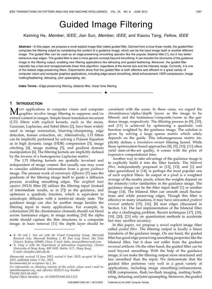
Fig. 1. Illustrations of the bilateral filtering process (left) and the guided filtering process (right).
It has been observed that these implicit filters are closely
related to the explicit ones. In [43], Elad shows that the
bilateral filter is one Jacobi iteration in solving the Gaussian
affinity matrix. The Hierarchical Local Adaptive Precondi-
tioners [41] and the Edge-Avoiding Wavelets [37] are
constructed in a similar manner. In this paper, we show
that the guided filter is closely related to the matting
Laplacian matrix [10].
2.3 Nonaverage Filters
Edge-preserving filtering can also be achieved by nonaver-
age filters. The median filter [2] is a well-known edge-aware
operator, and is a special case of local histogram filters [44].
Histogram filters have OðNÞ time implementations in a way
as the bilateral grid. The Total-Variation (TV) filters [45]
optimize an L1-regularized cost function, and are shown
equivalent to iterative median filtering [46]. The L1 cost
function can also be optimized via half-quadratic split [47],
alternating between a quadratic model and soft shrinkage
(thresholding). Recently, Paris et al. [48] proposed manip-
ulating the coefficients of the Laplacian Pyramid around
each pixel for edge-aware filtering. Xu et al. [49] propose
optimizing an L0-regularized cost function favoring piece-
wise constant solutions. The nonaverage filters are often
computationally expensive.
3 GUIDED FILTER
We first define a general linear translation-variant filtering
process, which involves a guidance image I, an filtering
input image p, and an output image q. Both I and p are
given beforehand according to the application, and they can
be identical. The filtering output at a pixel i is expressed as
a weighted average:
X
qi ¼
WijðIÞpj;
j
ð1Þ
where i and j are pixel indexes. The filter kernel Wij is a
function of the guidance image I and independent of p. This
filter is linear with respect to p.
An example of such a filter is the joint bilateral filter [14]
(Fig. 1 (left)). The bilateral filtering kernel W bf is given by
�
�
�
�
ij ðIÞ ¼ 1
W bf
Ki
exp �k xi � xj k2
exp �k Ii � Ij k2
ð2Þ
;
�2
s
�2
r
P
where x is the pixel coordinate and Ki is a normalizing
ij ¼ 1. The parameters �s
parameter to ensure that
and �r adjust the sensitivity of the spatial similarity and the
range (intensity/color) similarity, respectively. The joint
bilateral filter degrades to the original bilateral filter [1]
when I and p are identical.
j W bf
The implicit weighted-average filters (in Section 2.2)
optimize a quadratic function and solve a linear system in
this form:
Aq ¼ p;
ð3Þ
where q and p are N-by-1 vectors concatenating fqig and
fpig, respectively, and A is an N-by-N matrix only depends
on I. The solution to (3), i.e., q ¼ A�1p, has the same form as
(1), with Wij ¼ ðA�1Þij.
3.1 Definition
Now we define the guided filter. The key assumption of the
guided filter is a local linear model between the guidance I
and the filtering output q. We assume that q is a linear
transform of I in a window !k centered at the pixel k:
qi ¼ akIi þ bk;8i 2 !k;
ð4Þ
where ðak; bkÞ are some linear coefficients assumed to be
constant in !k. We use a square window of a radius r. This
local linear model ensures that q has an edge only if I has an
edge, because rq ¼ arI. This model has been proven
useful in image super-resolution [50], image matting [10],
and dehazing [11].
To determine the linear coefficients ðak; bkÞ, we need
constraints from the filtering input p. We model the output q
as the input p subtracting some unwanted components n
like noise/textures:
qi ¼ pi � ni:
ð5Þ
We seek a solution that minimizes the difference between q
and p while maintaining the linear model (4). Specifically,
we minimize the following cost function in the window !k:
ð6Þ
��
akIi þ bk � pi
Eðak; bkÞ ¼
X
2 þ �a2
k
:
�
�
i2!k
Here, � is a regularization parameter penalizing large ak. We
will
investigate its intuitive meaning in Section 3.2.
Equation (6) is the linear ridge regression model [51], [52]
and its solution is given by
�
P
1400
ak ¼ 1j!j
Iipi � �k �pk
i2!k
k þ �
�2
;
ð7Þ
IEEE TRANSACTIONS ON PATTERN ANALYSIS AND MACHINE INTELLIGENCE, VOL. 35, NO. 6,
JUNE 2013
bk ¼ �pk � ak�k:
ð8Þ
k are the mean and variance of I in !k, j!j is
Here, �k and �2
the number of pixels in !k, and �pk ¼ 1j!j
pi is the mean
of p in !k. Having obtained the linear coefficients ðak; bkÞ, we
can compute the filtering output qi by (4). Fig. 1 (right)
shows an illustration of the guided filtering process.
P
i2!k
However, a pixel i is involved in all the overlapping
windows !k that covers i, so the value of qi in (4) is not
identical when it is computed in different windows. A
simple strategy is to average all the possible values of qi. So
after computing ðak; bkÞ for all windows !k in the image, we
compute the filtering output by
ðakIi þ bkÞ:
ð9Þ
X
P
kji2!k
P
qi ¼ 1
j!j
ak ¼
k2!i
k2!i
k2!i
kji2!k
P
ak due to the symmetry of
Noticing that
the box window, we rewrite (9) by
P
qi ¼ �aiIi þ �bi;
ak and �bi ¼ 1j!j
ð10Þ
where �ai ¼ 1j!j
bk are the average
coefficients of all windows overlapping i. The averaging
strategy of overlapping windows is popular in image
denoising (see [53]) and is a building block of the very
successful BM3D algorithm [54].
With the modification in (10), rq is no longer scaling of rI
because the linear coefficients ð�ai; �biÞ vary spatially. But as
ð�ai; �biÞ are the output of a mean filter, their gradients can be
expected to be much smaller than that of I near strong edges.
In this situation we can still have rq � �arI, meaning that
abrupt intensity changes in I can be mostly preserved in q.
Equations (7), (8), and (10) are the definition of the
guided filter. A pseudocode is in Algorithm 1. In this
algorithm, fmean is a mean filter with a window radius r.
The abbreviations of correlation (corr), variance (var), and
covariance (cov) indicate the intuitive meaning of these
variables. We will discuss the fast implementation and the
computation details in Section. 4.
Algorithm 1. Guided Filter.
Input: filtering input image p, guidance image I, radius r,
regularization �
Output: filtering output q.
1: meanI ¼ fmeanðIÞ
meanp ¼ fmeanðpÞ
corrI ¼ fmeanðI: � IÞ
corrIp ¼ fmeanðI: � pÞ
2: varI ¼ corrI � meanI: � meanI
covIp ¼ corrIp � meanI: � meanp
3: a ¼ covIp:=ðvarI þ �Þ
b ¼ meanp � a: � meanI
4: meana ¼ fmeanðaÞ
meanb ¼ fmeanðbÞ
5: q ¼ meana: � I þ meanb
/� fmean is a mean filter with a wide variety of O(N) time
methods. �/
3.2 Edge-Preserving Filtering
Given the definition of the guided filter, we first study the
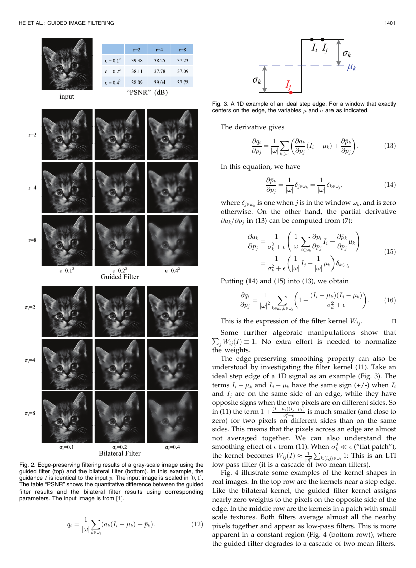
edge-preserving filtering property. Fig. 2 shows an example
of the guided filter with various sets of parameters. Here we
investigate the special case where the guide I is identical to
the filtering input p. We can see that the guided filter
behaves as an edge-preserving smoothing operator (Fig. 2).
The edge-preserving filtering property of the guided
filter can be explained intuitively as following. Consider the
case where I � p. In this case, ak ¼ �2
k=ð�2
k þ �Þ in (7) and
bk ¼ ð1 � akÞ�k. It is clear that if � ¼ 0, then ak ¼ 1 and
bk ¼ 0. If � > 0, we can consider two cases.
Case 1: “High variance.” If the image I changes a lot
within !k, we have �2
k � �, so ak � 1 and bk � 0.
Case 2: “Flat patch.” If the image I is almost constant in
!k, we have �2
k � �, so ak � 0 and bk � �k.
When ak and bk are averaged to get �ai and �bi, combined
in (10) to get the output, we have that if a pixel is in the
middle of a “high variance” area,
then its value is
unchanged (a � 1; b � 0; q � p), whereas if
is in the
middle of a “flat patch” area, its value becomes the average
of the pixels nearby (a � 0; b � �; q � ��).
it
More specifically, the criterion of a “flat patch” or a “high
variance” one is given by the parameter �. The patches with
variance (�2) much smaller than � are smoothed, whereas
those with variance much larger than � are preserved. The
effect of � in the guided filter is similar to the range variance
�2
in the bilateral filter (2): Both determine “what is an
r
edge/a high variance patch that should be preserved.”
Further, in a flat region the guided filter becomes a
cascade of two box mean filters whose radius is r. Cascades
of box filters are good approximations of Gaussian filters.
Thus, we empirically set up a “correspondence” between
the guided filter and the bilateral filter: r $ �s and � $ �2
r.
Fig. 2 shows the results of both filters using corresponding
parameters. The table “PSNR” in Fig. 2 shows the
quantitative difference between the guided filter results
and the bilateral filter results of the corresponding para-
meters.2 It is often considered as visually insensitive when
the PSNR � 40 dB [18].
3.3 Filter Kernel
It is easy to show that the relationships among I, p, and q,
P
given by (7), (8), and (10), are in the weighted-average form
as (1). In fact, ak in (7) can be rewritten as a weighted sum of
P
j AkjðIÞpj, where Aij are the weights only
p : ak ¼
dependent on I. For the same reason, we also have bk ¼
j BkjðIÞpj from (8) and qi ¼
j WijðIÞpj from (10). We can
�
prove that the kernel weights is explicitly expressed by
P
X
�
1 þ ðIi � �kÞðIj � �kÞ
k þ �
�2
WijðIÞ ¼ 1
j!j2
k:ði;jÞ2!k
:
ð11Þ
Proof. Due to the linear dependence between p and q, the
filter kernel is given by Wij ¼ @qi=@pj. Putting (8) into
(10) and eliminating b, we obtain
2. Note that we do not intend to approximate the bilateral filer, and the
bilateral filter results are not considered as “ground-truth.” So the “PSNR”
measure is just analogous to those used in the bilateral filter approximations
[18].
�
HE ET AL.: GUIDED IMAGE FILTERING
1401
Fig. 3. A 1D example of an ideal step edge. For a window that exactly
centers on the edge, the variables � and � are as indicated.
The derivative gives
X
�
�
@qi
@pj
¼ 1
j!j
k2!i
@ak
@pj
ðIi � �kÞ þ @ �pk
@pj
:
In this equation, we have
@ �pk
@pj
¼ 1
j!j �j2!k ¼ 1
j!j �k2!j ;
ð13Þ
ð14Þ
where �j2!k is one when j is in the window !k, and is zero
otherwise. On the other hand, the partial derivative
@ak=@pj in (13) can be computed from (7):
!
�
Ii � @ �pk
@pj
�k
j!j �k
�k2!j:
�
1 þ ðIi � �kÞðIj � �kÞ
:
k þ �
�2
ð15Þ
ð16Þ
@pi
@pj
X
�
1
j!j
j!j Ij � 1
1
�
i2!k
@ak
@pj
¼ 1
k þ �
�2
¼ 1
k þ �
�2
X
@qi
@pj
¼ 1
j!j2
k2!i;k2!j
Putting (14) and (15) into (13), we obtain
This is the expression of the filter kernel Wij.
tu
P
Some further algebraic manipulations show that
j WijðIÞ � 1. No extra effort
is needed to normalize
the weights.
The edge-preserving smoothing property can also be
understood by investigating the filter kernel (11). Take an
ideal step edge of a 1D signal as an example (Fig. 3). The
terms Ii � �k and Ij � �k have the same sign (+/-) when Ii
and Ij are on the same side of an edge, while they have
opposite signs when the two pixels are on different sides. So
in (11) the term 1 þ ðIi��kÞðIj��kÞ
is much smaller (and close to
zero) for two pixels on different sides than on the same
sides. This means that the pixels across an edge are almost
not averaged together. We can also understand the
k � � (“flat patch”),
smoothing effect of � from (11). When �2
the kernel becomes WijðIÞ � 1
1: This is an LTI
k:ði;jÞ2!k
j!j2
low-pass filter (it is a cascade of two mean filters).
P
kþ�
�2
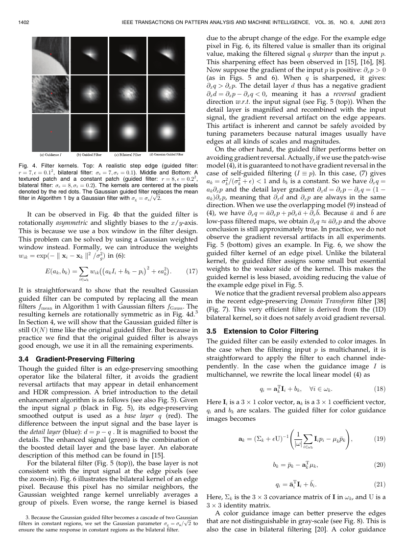
Fig. 4 illustrate some examples of the kernel shapes in
real images. In the top row are the kernels near a step edge.
Like the bilateral kernel, the guided filter kernel assigns
nearly zero weights to the pixels on the opposite side of the
edge. In the middle row are the kernels in a patch with small
scale textures. Both filters average almost all the nearby
pixels together and appear as low-pass filters. This is more
apparent in a constant region (Fig. 4 (bottom row)), where
the guided filter degrades to a cascade of two mean filters.
Fig. 2. Edge-preserving filtering results of a gray-scale image using the
guided filter (top) and the bilateral filter (bottom). In this example, the
guidance I is identical to the input p. The input image is scaled in ½0; 1.
The table “PSNR” shows the quantitative difference between the guided
filter
results using corresponding
parameters. The input image is from [1].
results and the bilateral
filter
X
qi ¼ 1
j!j
k2!i
ðakðIi � �kÞ þ �pkÞ:
ð12Þ
�
1402
IEEE TRANSACTIONS ON PATTERN ANALYSIS AND MACHINE INTELLIGENCE, VOL. 35, NO. 6,
JUNE 2013
due to the abrupt change of the edge. For the example edge
pixel in Fig. 6, its filtered value is smaller than its original
value, making the filtered signal q sharper than the input p.
This sharpening effect has been observed in [15], [16], [8].
Now suppose the gradient of the input p is positive: @xp > 0
(as in Figs. 5 and 6). When q is sharpened,
it gives:
@xq > @xp. The detail layer d thus has a negative gradient
@xd ¼ @xp � @xq < 0, meaning it has a reversed gradient
direction w.r.t. the input signal (see Fig. 5 (top)). When the
detail layer is magnified and recombined with the input
signal, the gradient reversal artifact on the edge appears.
This artifact is inherent and cannot be safely avoided by
tuning parameters because natural images usually have
edges at all kinds of scales and magnitudes.
k=ð�2
On the other hand, the guided filter performs better on
avoiding gradient reversal. Actually, if we use the patch-wise
model (4), it is guaranteed to not have gradient reversal in the
case of self-guided filtering (I � p). In this case, (7) gives
ak ¼ �2
k þ �Þ < 1 and bk is a constant. So we have @xq ¼
ak@xp and the detail layer gradient @xd ¼ @xp � @xq ¼ ð1 �
akÞ@xp, meaning that @xd and @xp are always in the same
direction. When we use the overlapping model (9) instead of
(4), we have @xq ¼ �a@xp þ p@x �a þ @x �b. Because �a and �b are
low-pass filtered maps, we obtain @xq � �a@xp and the above
conclusion is still approximately true. In practice, we do not
observe the gradient reversal artifacts in all experiments.
Fig. 5 (bottom) gives an example. In Fig. 6, we show the
guided filter kernel of an edge pixel. Unlike the bilateral
kernel, the guided filter assigns some small but essential
weights to the weaker side of the kernel. This makes the
guided kernel is less biased, avoiding reducing the value of
the example edge pixel in Fig. 5.
We notice that the gradient reversal problem also appears
in the recent edge-preserving Domain Transform filter [38]
(Fig. 7). This very efficient filter is derived from the (1D)
bilateral kernel, so it does not safely avoid gradient reversal.
3.5 Extension to Color Filtering
The guided filter can be easily extended to color images. In
the case when the filtering input p is multichannel, it is
straightforward to apply the filter to each channel inde-
pendently. In the case when the guidance image I is
multichannel, we rewrite the local linear model (4) as
qi ¼ aT
k Ii þ bk;
ð18Þ
Here Ii is a 3 � 1 color vector, ak is a 3 � 1 coefficient vector,
qi and bk are scalars. The guided filter for color guidance
images becomes
8i 2 !k:
!
X
ak ¼ ð�k þ �UÞ�1
1
j!j
i2!k
Iipi � �k �pk
;
bk ¼ �pk � aT
k �k;
ð19Þ
ð20Þ
ð21Þ
Here, �k is the 3 � 3 covariance matrix of I in !k, and U is a
3 � 3 identity matrix.
i Ii þ �bi:
qi ¼ �aT
A color guidance image can better preserve the edges
that are not distinguishable in gray-scale (see Fig. 8). This is
also the case in bilateral filtering [20]. A color guidance
Fig. 4. Filter kernels. Top: A realistic step edge (guided filter:
r ¼ 7; � ¼ 0:12, bilateral filter: �s ¼ 7; �r ¼ 0:1). Middle and Bottom: A
textured patch and a constant patch (guided filter: r ¼ 8; � ¼ 0:22,
bilateral filter: �s ¼ 8; �r ¼ 0:2). The kernels are centered at the pixels
p
denoted by the red dots. The Gaussian guided filter replaces the mean
filter in Algorithm 1 by a Gaussian filter with �g ¼ �s=
ffiffiffi
2
.
It can be observed in Fig. 4b that the guided filter is
rotationally asymmetric and slightly biases to the x/y-axis.
This is because we use a box window in the filter design.
This problem can be solved by using a Gaussian weighted
��
window instead. Formally, we can introduce the weights
gÞ in (6):
wik ¼ expð� k xi � xk k2 =�2
akIi þ bk � pi
Eðak; bkÞ ¼
2 þ �a2
X
ð17Þ
wik
�
�
:
k
i2!k
It is straightforward to show that the resulted Gaussian
guided filter can be computed by replacing all the mean
filters fmean in Algorithm 1 with Gaussian filters fGauss. The
resulting kernels are rotationally symmetric as in Fig. 4d.3
In Section 4, we will show that the Gaussian guided filter is
still OðNÞ time like the original guided filter. But because in
practice we find that the original guided filter is always
good enough, we use it in all the remaining experiments.
3.4 Gradient-Preserving Filtering
Though the guided filter is an edge-preserving smoothing
operator like the bilateral filter,
it avoids the gradient
reversal artifacts that may appear in detail enhancement
and HDR compression. A brief introduction to the detail
enhancement algorithm is as follows (see also Fig. 5). Given
the input signal p (black in Fig. 5), its edge-preserving
is used as a base layer q (red). The
smoothed output
difference between the input signal and the base layer is
the detail layer (blue): d ¼ p � q . It is magnified to boost the
details. The enhanced signal (green) is the combination of
the boosted detail layer and the base layer. An elaborate
description of this method can be found in [15].
For the bilateral filter (Fig. 5 (top)), the base layer is not
consistent with the input signal at the edge pixels (see
the zoom-in). Fig. 6 illustrates the bilateral kernel of an edge
pixel. Because this pixel has no similar neighbors, the
Gaussian weighted range kernel unreliably averages a
group of pixels. Even worse, the range kernel is biased
3. Because the Gaussian guided filter becomes a cascade of two Gaussian
to
filters in constant regions, we set the Gaussian parameter �g ¼ �s=
ensure the same response in constant regions as the bilateral filter.
2
ffiffiffi
p
�
HE ET AL.: GUIDED IMAGE FILTERING
1403
Fig. 8. Guided filtering results guided by the color image (b) and guided
by its gray-scale version (c). The result in (c) has halos because the
edge is not undistinguishable in gray-scale.
Fig. 9. Structure-transferring filtering.
image is also essential
in the matting/feathering and
dehazing applications, as we show later, because the local
linear model is more likely to be valid in the RGB color
space than in gray-scale [10].
3.6 Structure-Transferring Filtering
Interestingly, the guided filter is not simply a smoothing
filter. Due to the local linear model of q ¼ aI þ b, the output q
is locally a scaling (plus an offset) of the guidance I. This
makes it possible to transfer structure from the guidance I to
the output q, even if the filtering input p is smooth (see Fig. 9).
To show an example of structure-transferring filtering,
we introduce an application of guided feathering: A binary
mask is refined to appear an alpha matte near the object
boundaries (Fig. 10). The binary mask can be obtained from
graph-cut or other segmentation methods, and is used as the
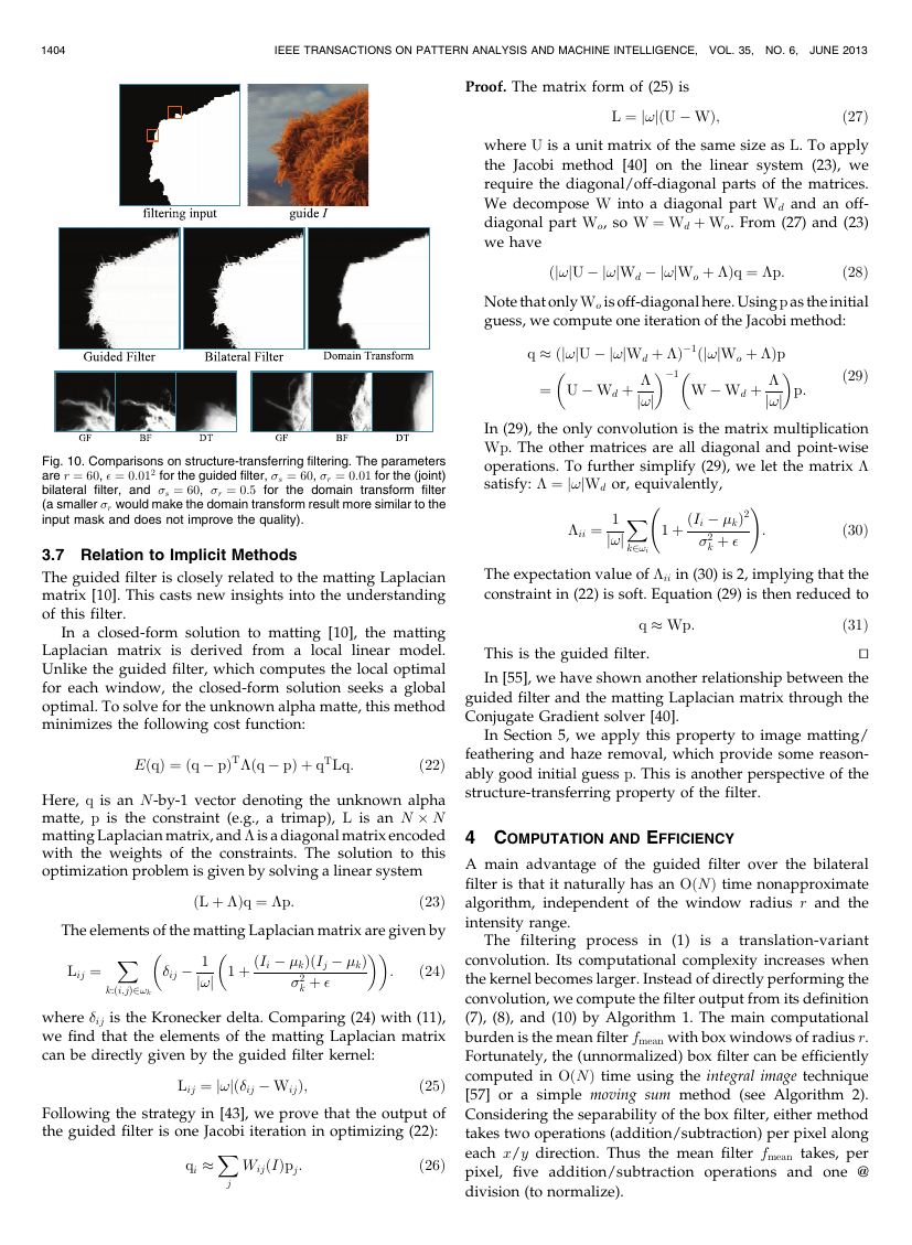
filter input p. The guidance I is the color image. Fig. 10 shows
the behaviors of three filters: guided filter, (joint) bilateral
filter, and a recent domain transform filter [38]. We observe
that the guided filter faithfully recovers the hair, even
though the filtering input p is binary and very rough. The
bilateral filter may lose some thin structures (see zoom-in).
This is because the bilateral filer is guided by pixel-wise
color difference, whereas the guided filter has a patch-wise
model. We also observe that the domain transform filter
does not have a good structure-transferring ability and
simply smooths the result. This is because this filter is based
on geodesic distance of pixels, and its output is a series of 1D
box filters with adaptive spans [38].
The structure-transferring filtering is an important
property of the guided filter. It enables new filtering-based
applications, including feathering/matting and dehazing
(Section 5). It also enables high-quality filtering-based stereo
matching methods in [23] and [24].
Fig. 5. 1D illustration for detail enhancement. See the text for explanation.
Fig. 6. The filtering results and the filter kernels at a pixel on a clean
edge. In this example, the edge height is 1 and the edge slope spans
20 pixels. The parameters are r ¼ 30; � ¼ 0:152 for the guided filter and
�s ¼ 30; �r ¼ 0:15 for the bilateral filter.
Fig. 7. Gradient reversal artifacts in the domain transform filter [38].
�
1404
IEEE TRANSACTIONS ON PATTERN ANALYSIS AND MACHINE INTELLIGENCE, VOL. 35, NO. 6,
JUNE 2013
Proof. The matrix form of (25) is
L ¼ j!jðU � WÞ;
ð27Þ
where U is a unit matrix of the same size as L. To apply
the Jacobi method [40] on the linear system (23), we
require the diagonal/off-diagonal parts of the matrices.
We decompose W into a diagonal part Wd and an off-
diagonal part Wo, so W ¼ Wd þ Wo. From (27) and (23)
we have
ðj!jU � j!jWd � j!jWo þ �Þq ¼ �p:
ð28Þ
Note that only Wo is off-diagonal here. Using p as the initial
guess, we compute one iteration of the Jacobi method:
�
�
�
q � ðj!jU � j!jWd þ �Þ�1ðj!jWo þ �Þp
¼ U � Wd þ �
W � Wd þ �
j!j
j!j
�
�1
p:
ð29Þ
In (29), the only convolution is the matrix multiplication
Wp. The other matrices are all diagonal and point-wise
operations. To further simplify (29), we let the matrix �
satisfy: � ¼ j!jWd or, equivalently,
!
X
�ii ¼ 1
j!j
k2!i
1 þ ðIi � �kÞ2
k þ �
�2
:
ð30Þ
The expectation value of �ii in (30) is 2, implying that the
constraint in (22) is soft. Equation (29) is then reduced to
ð31Þ
tu
In [55], we have shown another relationship between the
guided filter and the matting Laplacian matrix through the
Conjugate Gradient solver [40].
This is the guided filter.
q � Wp:
In Section 5, we apply this property to image matting/
feathering and haze removal, which provide some reason-
ably good initial guess p. This is another perspective of the
structure-transferring property of the filter.
4 COMPUTATION AND EFFICIENCY
A main advantage of the guided filter over the bilateral
filter is that it naturally has an OðNÞ time nonapproximate
algorithm, independent of the window radius r and the
intensity range.
The filtering process in (1) is a translation-variant
convolution. Its computational complexity increases when
the kernel becomes larger. Instead of directly performing the
convolution, we compute the filter output from its definition
(7), (8), and (10) by Algorithm 1. The main computational
burden is the mean filter fmean with box windows of radius r.
Fortunately, the (unnormalized) box filter can be efficiently
computed in OðNÞ time using the integral image technique
[57] or a simple moving sum method (see Algorithm 2).
Considering the separability of the box filter, either method
takes two operations (addition/subtraction) per pixel along
each x/y direction. Thus the mean filter fmean takes, per
pixel, five addition/subtraction operations and one @
division (to normalize).
Fig. 10. Comparisons on structure-transferring filtering. The parameters
are r ¼ 60, � ¼ 0:012 for the guided filter, �s ¼ 60, �r ¼ 0:01 for the (joint)
filter, and �s ¼ 60, �r ¼ 0:5 for the domain transform filter
bilateral
(a smaller �r would make the domain transform result more similar to the
input mask and does not improve the quality).
3.7 Relation to Implicit Methods
The guided filter is closely related to the matting Laplacian
matrix [10]. This casts new insights into the understanding
of this filter.
In a closed-form solution to matting [10], the matting
Laplacian matrix is derived from a local
linear model.
Unlike the guided filter, which computes the local optimal
for each window, the closed-form solution seeks a global
optimal. To solve for the unknown alpha matte, this method
minimizes the following cost function:
EðqÞ ¼ ðq � pÞT�ðq � pÞ þ qTLq:
ð22Þ
Here, q is an N-by-1 vector denoting the unknown alpha
matte, p is the constraint (e.g., a trimap), L is an N � N
matting Laplacian matrix, and � is a diagonal matrix encoded
with the weights of the constraints. The solution to this
optimization problem is given by solving a linear system
The elements of the matting Laplacian matrix are given by
ðL þ �Þq ¼ �p:
�
�
j!j 1 þ ðIi � �kÞðIj � �kÞ
k þ �
�2
�
ð23Þ
ð24Þ
:
�
X
Lij ¼
k:ði;jÞ2!k
�ij � 1
where �ij is the Kronecker delta. Comparing (24) with (11),
we find that the elements of the matting Laplacian matrix
can be directly given by the guided filter kernel:
Lij ¼ j!jð�ij � WijÞ;
ð25Þ
Following the strategy in [43], we prove that the output of
the guided filter is one Jacobi iteration in optimizing (22):
ð26Þ
WijðIÞpj:
qi �
X
j
�



 2023年江西萍乡中考道德与法治真题及答案.doc
 2012年重庆南川中考生物真题及答案.doc
 2013年江西师范大学地理学综合及文艺理论基础考研真题.doc
 2020年四川甘孜小升初语文真题及答案I卷.doc
 2020年注册岩土工程师专业基础考试真题及答案.doc
 2023-2024学年福建省厦门市九年级上学期数学月考试题及答案.doc
 2021-2022学年辽宁省沈阳市大东区九年级上学期语文期末试题及答案.doc
 2022-2023学年北京东城区初三第一学期物理期末试卷及答案.doc
 2018上半年江西教师资格初中地理学科知识与教学能力真题及答案.doc
 2012年河北国家公务员申论考试真题及答案-省级.doc
 2020-2021学年江苏省扬州市江都区邵樊片九年级上学期数学第一次质量检测试题及答案.doc
 2022下半年黑龙江教师资格证中学综合素质真题及答案.doc