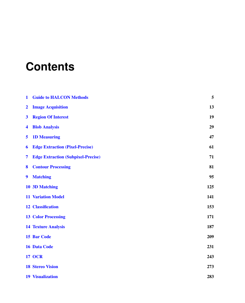
1 Guide to HALCON Methods
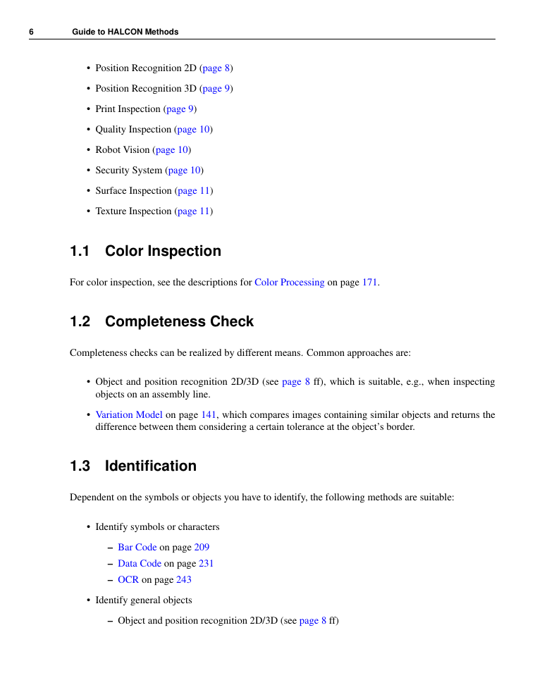
1.1 Color Inspection
1.2 Completeness Check
1.3 Identification
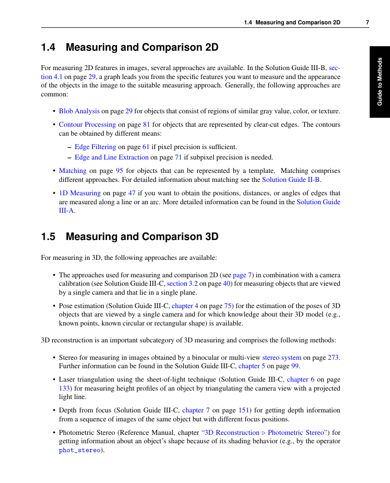
1.4 Measuring and Comparison 2D
1.5 Measuring and Comparison 3D
1.6 Object Recognition 2D
1.7 Object Recognition 3D
1.8 Position Recognition 2D
1.9 Position Recognition 3D
1.10 Print Inspection
1.11 Quality Inspection
1.12 Robot Vision
1.13 Security System
1.14 Surface Inspection
1.15 Texture Inspection
2 Image Acquisition
2.1 Basic Concept
2.1.1 Open Image Acquisition Device
2.1.2 Acquire Image(s)
2.1.3 Close Image Acquisition Device
2.1.4 A First Example
2.2 Extended Concept
2.2.1 Open Image Acquisition Device
2.2.2 Set Parameters
2.2.3 Acquire Image(s)
2.3 Programming Examples
2.4 Selecting Operators
2.4.1 Open Image Acquisition Device
2.4.2 Set Parameters
2.4.3 Acquire Image(s)
2.4.4 Close Image Acquisition Device
2.5 Tips & Tricks
2.5.1 Direct Access to External Images in Memory
2.5.2 Unsupported Image Acquisition Devices
3 Region Of Interest
3.1 Basic Concept
3.1.1 Create Region
3.1.2 Create ROI
3.1.3 A First Example
3.2 Extended Concept
3.2.1 Segment Image(s)
3.2.2 Draw Region
3.2.3 Create Region
3.2.4 Process Regions
3.2.5 Align ROIs Or Images
3.2.6 Create ROI
3.2.7 Visualize Results
3.3 Programming Examples
3.3.1 Processing inside a User Defined Region
3.3.2 Interactive Partial Filtering of an Image
3.3.3 Inspecting the Contours of a Tool
3.4 Selecting Operators
3.4.1 Segment Image(s)
3.4.2 Draw Region
3.4.3 Create Region
3.4.4 Process Regions
3.4.5 Align ROIs Or Images
3.4.6 Create ROI
3.4.7 Visualize Results
3.5 Relation to Other Methods
3.6 Tips & Tricks
3.6.1 Reuse ROI
3.6.2 Effect of ROI Shape on Speed Up
3.7 Advanced Topics
3.7.1 Filter masks and ROIs
3.7.2 Binary Images
4 Blob Analysis
4.1 Basic Concept
4.1.1 Acquire Image(s)
4.1.2 Segment Image(s)
4.1.3 Extract Features
4.1.4 A First Example
4.2 Extended Concept
4.2.1 Use Region Of Interest
4.2.2 Align ROIs Or Images
4.2.3 Rectify Image(s)
4.2.4 Preprocess Image(s) (Filtering)
4.2.5 Extract Segmentation Parameters
4.2.6 Segment Image(s)
4.2.7 Process Regions
4.2.8 Extract Features
4.2.9 Transform Results Into World Coordinates
4.2.10 Visualize Results
4.3 Programming Examples
4.3.1 Crystals
4.3.2 Atoms
4.3.3 Analyzing Particles
4.3.4 Extracting Forest Features from Color Infrared Image
4.3.5 Checking a Boundary for Fins
4.3.6 Bonding Balls
4.3.7 Surface Scratches
4.4 Selecting Operators
4.4.1 Acquire Image(s)
4.4.2 Use Region Of Interest
4.4.3 Align ROIs Or Images
4.4.4 Rectify Image(s)
4.4.5 Preprocess Image(s) (Filtering)
4.4.6 Extract Segmentation Parameters
4.4.7 Segment Image(s)
4.4.8 Process Regions
4.4.9 Extract Features
4.4.10 Transform Results Into World Coordinates
4.4.11 Visualize Results
4.5 Relation to Other Methods
4.5.1 Methods that are Useful for Blob Analysis
4.5.2 Methods that are Using Blob Analysis
4.5.3 Alternatives to Blob Analysis
4.6 Tips & Tricks
4.6.1 Connected Components
4.6.2 Speed Up
4.7 Advanced Topics
4.7.1 Line Scan Cameras
4.7.2 High Accuracy
5 1D Measuring
5.1 Basic Concept
5.1.1 Acquire Image(s)
5.1.2 Create Measure Object
5.1.3 Measure
5.1.4 Destroy Measure Object
5.2 Extended Concept
5.2.1 Radiometrically Calibrate Image(s)
5.2.2 Align ROIs Or Images
5.2.3 Rectify Image(s)
5.2.4 Create Measure Object
5.2.5 Transform Results Into World Coordinates
5.2.6 Visualize Results
5.3 Programming Examples
5.3.1 Inspecting a Fuse
5.3.2 Inspect Cast Part
5.3.3 Inspecting an IC Using Fuzzy Measuring
5.3.4 Measuring Leads of a Moving IC
5.3.5 Inspect IC
5.4 Selecting Operators
5.4.1 Acquire Image(s)
5.4.2 Radiometrically Calibrate Image(s)
5.4.3 Align ROIs Or Images
5.4.4 Rectify Image(s)
5.4.5 Create Measure Object
5.4.6 Measure
5.4.7 Transform Results Into World Coordinates
5.4.8 Visualize Results
5.4.9 Destroy Measure Object
5.5 Relation to Other Methods
5.5.1 Alternatives to 1D Measuring
5.6 Tips & Tricks
5.6.1 Suppress Clutter or Noise
5.6.2 Reuse Measure Object
5.6.3 Use an Absolute Gray Value Threshold
5.7 Advanced Topics
5.7.1 Fuzzy Measuring
5.7.2 Evaluation of Gray Values
6 Edge Extraction (Pixel-Precise)
6.1 Basic Concept
6.1.1 Acquire Image(s)
6.1.2 Filter Image
6.1.3 Extract Edges
6.1.4 Process Edges
6.1.5 A First Example
6.2 Extended Concept
6.2.1 Use Region Of Interest
6.2.2 Filter Image
6.2.3 Extract Edges
6.2.4 Process Edges
6.2.5 Visualize Results
6.3 Programming Examples
6.3.1 Aerial Image Interpretation
6.3.2 Segmenting a Color Image
6.4 Selecting Operators
6.4.1 Acquire Image(s)
6.4.2 Use Region Of Interest
6.4.3 Filter Image
6.4.4 Extract Edges
6.4.5 Process Edges
6.4.6 Visualize Results
6.5 Relation to Other Methods
6.5.1 Alternatives to Edge Extraction (Pixel-Precise)
6.6 Tips & Tricks
6.6.1 Speed Up
7 Edge Extraction (Subpixel-Precise)
7.1 Basic Concept
7.1.1 Acquire Image(s)
7.1.2 Extract Edges Or Lines
7.1.3 A First Example
7.2 Extended Concept
7.2.1 Radiometrically Calibrate Image(s)
7.2.2 Use Region Of Interest
7.2.3 Extract Edges Or Lines
7.2.4 Determine Contour Attributes
7.2.5 Process XLD Contours
7.2.6 Transform Results Into World Coordinates
7.2.7 Visualize Results
7.3 Programming Examples
7.3.1 Measuring the Diameter of Drilled Holes
7.3.2 Angiography
7.4 Selecting Operators
7.4.1 Acquire Image(s)
7.4.2 Radiometrically Calibrate Image(s)
7.4.3 Use Region Of Interest
7.4.4 Extract Edges Or Lines
7.4.5 Determine Contour Attributes
7.4.6 Process XLD Contours
7.4.7 Transform Results Into World Coordinates
7.4.8 Visualize Results
7.5 Relation to Other Methods
7.5.1 Alternatives to Edge Extraction (Subpixel-Precise)
8 Contour Processing
8.1 Basic Concept
8.1.1 Create XLD Contours
8.1.2 Process XLD Contours
8.1.3 Perform Fitting
8.1.4 Extract Features
8.1.5 A First Example
8.2 Extended Concept
8.2.1 Create XLD Contours
8.2.2 Process XLD Contours
8.2.3 Perform Fitting
8.2.4 Transform Results Into World Coordinates
8.2.5 Extract Features
8.2.6 Convert And Access XLD Contours
8.2.7 Visualize Results
8.3 Programming Examples
8.3.1 Measuring Lines and Arcs
8.3.2 Close gaps in a contour
8.3.3 Extract Roads
8.4 Selecting Operators
8.4.1 Create XLD Contours
8.4.2 Process XLD Contours
8.4.3 Perform Fitting
8.4.4 Transform Results Into World Coordinates
8.4.5 Extract Features
8.4.6 Convert And Access XLD Contours
8.4.7 Visualize Results
8.5 Relation to Other Methods
8.5.1 Alternatives to Contour Processing
8.6 Advanced Topics
8.6.1 Line Scan Cameras
9 Matching
9.1 Basic Concept
9.1.1 Acquire Image(s)
9.1.2 Create (Train) Model
9.1.3 Find Model
9.1.4 Destroy Model
9.1.5 A First Example
9.2 Extended Concept
9.2.1 Radiometrically Calibrate Image(s)
9.2.2 Rectify Image(s)
9.2.3 Use Region Of Interest
9.2.4 Determine Training Parameters
9.2.5 Create (Train) Model
9.2.6 Find Model
9.2.7 Visualize Results
9.3 Programming Examples
9.3.1 Creating a Model for the ``Green Dot''
9.3.2 Locating ``Green Dots''
9.3.3 Distinguishing coins
9.3.4 Locate Components on a PCB
9.3.5 Check the State of a Dip Switch
9.3.6 Locating a Pipe Wrench in Different States
9.3.7 Creating a Mosaic Image
9.3.8 Locate Brochure Pages
9.3.9 Locate Road Signs
9.4 Selecting Operators
9.4.1 Acquire Image(s)
9.4.2 Radiometrically Calibrate Image(s)
9.4.3 Rectify Image(s)
9.4.4 Use Region Of Interest
9.4.5 Determine Training Parameters
9.4.6 Create (Train) Model
9.4.7 Find Model
9.4.8 Visualize Results
9.4.9 Destroy Model
9.5 Relation to Other Methods
9.5.1 Methods that are Using Matching
9.5.2 Alternatives to Matching
9.6 Tips & Tricks
9.6.1 Speed Up
9.7 Advanced Topics
9.7.1 High Accuracy
9.7.2 Use Timeout
10 3D Matching
10.1 Basic Concept
10.1.1 Access 3D Object Model
10.1.2 Create Approach-Specific 3D Model
10.1.3 Destroy 3D Object Model
10.1.4 Acquire Search Data
10.1.5 Find Approach-Specific 3D Model
10.1.6 Destroy Approach-Specific 3D Model
10.1.7 A First Example
10.2 Extended Concept
10.2.1 Inspect 3D Object Model
10.2.2 Inspect Approach-Specific 3D Model
10.2.3 Re-use Approach-Specific 3D Model
10.2.4 Use Region Of Interest
10.2.5 Visualize Results
10.3 Programming Examples
10.3.1 Recognize 3D Clamps and Their Poses in Images
10.3.2 Recognize Pipe Joints and Their Poses in a 3D Scene
10.4 Selecting Operators
10.4.1 Access 3D Object Model
10.4.2 Inspect 3D Object Model
10.4.3 Create Approach-Specific 3D Model
10.4.4 Destroy 3D Object Model
10.4.5 Inspect Approach-Specific 3D Model
10.4.6 Re-use Approach-Specific 3D Model
10.4.7 Acquire Search Data
10.4.8 Use Region Of Interest
10.4.9 Find Approach-Specific 3D Model
10.4.10 Visualize Results
10.4.11 Destroy Approach-Specific 3D Model
10.5 Relation to Other Methods
10.5.1 Alternatives to 3D Matching
11 Variation Model
11.1 Basic Concept
11.1.1 Acquire Image(s)
11.1.2 Create Variation Model
11.1.3 Align ROIs Or Images
11.1.4 Train Variation Model
11.1.5 Prepare Variation Model
11.1.6 Compare Variation Model
11.1.7 Destroy Variation Model
11.1.8 A First Example
11.2 Extended Concept
11.2.1 Check Model Quality
11.2.2 Clear Training Data
11.2.3 Visualize Results
11.3 Programming Examples
11.3.1 Inspect a Printed Logo Using a Single Reference Image
11.3.2 Inspect a Printed Logo under Varying Illumination
11.4 Selecting Operators
11.4.1 Acquire Image(s)
11.4.2 Create Variation Model
11.4.3 Align ROIs Or Images
11.4.4 Train Variation Model
11.4.5 Check Model Quality
11.4.6 Prepare Variation Model
11.4.7 Clear Training Data
11.4.8 Compare Variation Model
11.4.9 Visualize Results
11.4.10 Destroy Variation Model
12 Classification
12.1 Basic Concept
12.1.1 Acquire Image(s)
12.1.2 Create Classifier
12.1.3 Train Classifier
12.1.4 Classify Data
12.1.5 Destroy Classifier
12.1.6 A First Example
12.2 Extended Concept
12.2.1 Train Classifier
12.2.2 Re-use Training Samples
12.2.3 Re-use Classifier
12.2.4 Evaluate Classifier
12.2.5 Visualize Results
12.3 Programming Examples
12.3.1 Inspection of Plastic Meshes via Texture Classification
12.3.2 Classification with Overlapping Classes
12.4 Selecting Operators
12.4.1 Acquire Image(s)
12.4.2 Create Classifier
12.4.3 Train Classifier
12.4.4 Re-use Training Samples
12.4.5 Re-use Classifier
12.4.6 Evaluate Classifier
12.4.7 Classify Data
12.4.8 Visualize Results
12.4.9 Destroy Classifier
12.5 Relation to Other Methods
12.5.1 Methods that are Useful for Classification
12.5.2 Methods that are Using Classification
12.5.3 Alternatives to Classification
12.6 Tips & Tricks
12.6.1 OCR for General Classification
12.7 Advanced Topics
12.7.1 Selection of Training Samples
13 Color Processing
13.1 Basic Concept
13.1.1 Acquire Image(s)
13.1.2 Decompose Channels
13.1.3 Process Image (Channels)
13.1.4 A First Example
13.2 Extended Concept
13.2.1 Demosaick Bayer Pattern
13.2.2 Transform Color Space
13.2.3 Train Colors
13.2.4 Use Region Of Interest
13.2.5 Classify Colors
13.2.6 Compose Channels
13.2.7 Visualize Results
13.3 Programming Examples
13.3.1 Robust Color Extraction
13.3.2 Sorting Fuses
13.3.3 Completeness Check of Colored Game Pieces
13.3.4 Inspect Power Supply Cables
13.3.5 Locating Board Components by Color
13.4 Selecting Operators
13.4.1 Acquire Image(s)
13.4.2 Demosaick Bayer Pattern
13.4.3 Decompose Channels
13.4.4 Transform Color Space
13.4.5 Train Colors
13.4.6 Use Region Of Interest
13.4.7 Process Image (Channels)
13.4.8 Classify Colors
13.4.9 Compose Channels
13.4.10 Visualize Results
13.5 Tips & Tricks
13.5.1 Speed Up
13.6 Advanced Topics
13.6.1 Color Edge Extraction
13.6.2 Color Line Extraction
14 Texture Analysis
14.1 Basic Concept
14.1.1 Acquire Image(s)
14.1.2 Apply Texture Filter
14.1.3 Compute Features
14.1.4 A First Example
14.2 Extended Concept
14.2.1 Rectify Image(s)
14.2.2 Scale Down Image(s)
14.2.3 Use Region Of Interest
14.2.4 Align ROIs Or Images
14.2.5 Apply Texture Filter
14.2.6 Compute Features
14.2.7 Visualize Results
14.2.8 Use Results
14.3 Programming Examples
14.3.1 Detect Defects in a Texture with Novelty Detection
14.3.2 Detect Defects in a Web Using Dynamic Thresholding
14.3.3 Classification of Different Types of Wood
14.4 Selecting Operators
14.4.1 Acquire Image(s)
14.4.2 Rectify Image(s)
14.4.3 Scale Down Image(s)
14.4.4 Use Region Of Interest
14.4.5 Align ROIs Or Images
14.4.6 Apply Texture Filter
14.4.7 Compute Features
14.4.8 Visualize Results
14.4.9 Use Results
14.5 Relation to Other Methods
14.5.1 Methods that are Using Texture Analysis
14.6 Advanced Topics
14.6.1 Fast Fourier Transform (FFT)
14.6.2 Texture Analysis in Color Images
14.7 More Information About Texture Features
14.7.1 Entropy and Anisotropy ([file:../reference/reference_hdevelop.pdf]entropy_gray)
14.7.2 Cooccurrence Matrix ([file:../reference/reference_hdevelop.pdf]gen_cooc_matrix)
14.7.3 Features of the Cooccurrence Matrix
14.8 More Information About Texture Filtering
14.8.1 The Laws Filter ([file:../reference/reference_hdevelop.pdf]texture_laws)
15 Bar Code
15.1 Basic Concept
15.1.1 Acquire Image(s)
15.1.2 Create Bar Code Model
15.1.3 Read Bar Code(s)
15.1.4 Destroy Bar Code Model
15.1.5 A First Example
15.2 Extended Concept
15.2.1 Use Region Of Interest
15.2.2 Preprocess Image(s)
15.2.3 Rectify Image(s)
15.2.4 Create Bar Code Model
15.2.5 Adjust Bar Code Model
15.2.6 Read Bar Code(s)
15.2.7 Check Print Quality
15.2.8 Visualize Results
15.3 Programming Examples
15.3.1 How to Read Difficult Barcodes
15.3.2 Reading a Bar Code on a CD
15.3.3 Checking Bar Code Print Quality
15.4 Selecting Operators
15.4.1 Acquire Image(s)
15.4.2 Use Region Of Interest
15.4.3 Preprocess Image(s)
15.4.4 Rectify Image(s)
15.4.5 Create Bar Code Model
15.4.6 Adjust Bar Code Model
15.4.7 Read Bar Code(s)
15.4.8 Destroy Bar Code Model
15.4.9 Check Print Quality
15.4.10 Visualize Results
15.5 Relation to Other Methods
15.5.1 Alternatives to Bar Code
15.6 Advanced Topics
15.6.1 Use Timeout
16 Data Code
16.1 Basic Concept
16.1.1 Acquire Image(s)
16.1.2 Create Data Code Model
16.1.3 Read Data Code(s)
16.1.4 Destroy Data Code Model
16.1.5 A First Example
16.2 Extended Concept
16.2.1 Acquire Image(s)
16.2.2 Rectify Image(s)
16.2.3 Create Data Code Model
16.2.4 Optimize Model
16.2.5 Train Model
16.2.6 Use Region Of Interest
16.2.7 Read Data Code(s)
16.2.8 Inspect Data Code(s)
16.2.9 Check Print Quality
16.2.10 Visualize Results
16.3 Programming Examples
16.3.1 Training a Data Code Model
16.3.2 Reading 2D Data Codes on Chips
16.4 Selecting Operators
16.4.1 Acquire Image(s)
16.4.2 Rectify Image(s)
16.4.3 Create Data Code Model
16.4.4 Optimize Model
16.4.5 Train Model
16.4.6 Use Region Of Interest
16.4.7 Read Data Code(s)
16.4.8 Inspect Data Code(s)
16.4.9 Check Print Quality
16.4.10 Visualize Results
16.4.11 Destroy Data Code Model
16.5 Advanced Topics
16.5.1 Use Timeout
17 OCR
17.1 Basic Concept
17.1.1 Acquire Image(s)
17.1.2 Segment Image(s)
17.1.3 Train OCR
17.1.4 Read Symbol
17.1.5 Destroy Classifier
17.1.6 A First Example
17.2 Extended Concept
17.2.1 Use Region Of Interest
17.2.2 Align ROIs Or Images
17.2.3 Rectify Image(s)
17.2.4 Preprocess Image(s) (Filtering)
17.2.5 Extract Segmentation Parameters
17.2.6 Segment Image(s)
17.2.7 Train OCR
17.2.8 Read Symbol
17.2.9 Visualize Results
17.3 Programming Examples
17.3.1 Generating a Training File
17.3.2 Creating and Training an OCR Classifier
17.3.3 Reading Numbers
17.3.4 "Best Before" Date
17.3.5 Reading Engraved Text
17.3.6 Reading Forms
17.3.7 Segment and Select Characters
17.3.8 Syntactic and Lexicon-Based Auto-Correction of OCR Results
17.4 Selecting Operators
17.4.1 Acquire Image(s)
17.4.2 Use Region Of Interest
17.4.3 Align ROIs Or Images
17.4.4 Rectify Image(s)
17.4.5 Preprocess Image(s) (Filtering)
17.4.6 Extract Segmentation Parameters
17.4.7 Segment Image(s)
17.4.8 Train OCR
17.4.9 Read Symbol
17.4.10 Visualize Results
17.4.11 Destroy Classifier
17.5 Relation to Other Methods
17.5.1 Alternatives to OCR
17.6 Tips & Tricks
17.6.1 Composed Symbols
17.7 Advanced Topics
17.7.1 Line Scan Cameras
17.7.2 Circular Prints
17.7.3 OCR Features
17.8 Pretrained OCR Fonts
17.8.1 Nomenclature for the Ready-to-Use OCR Fonts
17.8.2 Ready-to-Use OCR Font 'Document'
17.8.3 Ready-to-Use OCR Font 'DotPrint'
17.8.4 Ready-to-Use OCR Font 'HandWritten_0-9'
17.8.5 Ready-to-Use OCR Font 'Industrial'
17.8.6 Ready-to-Use OCR Font 'MICR'
17.8.7 Ready-to-Use OCR Font 'OCR-A'
17.8.8 Ready-to-Use OCR Font 'OCR-B'
17.8.9 Ready-to-Use OCR Font 'Pharma'
17.8.10 Ready-to-Use OCR Font 'SEMI'
18 Stereo Vision
18.1 Basic Concept
18.1.1 Calibrate Stereo Camera System
18.1.2 Acquire Image(s)
18.1.3 Rectify Image(s)
18.1.4 Reconstruct 3D Information
18.2 Extended Concept
18.2.1 Use Region Of Interest
18.2.2 Transform Results Into World Coordinates
18.2.3 Visualize Results
18.3 Programming Examples
18.3.1 Segment the Components of a Board With Binocular Stereo
18.3.2 Reconstruct the Surface of Pipe Joints With Multi-View Stereo
18.4 Selecting Operators
18.4.1 Calibrate Stereo Camera System
18.4.2 Acquire Image(s)
18.4.3 Rectify Image(s)
18.4.4 Use Region Of Interest
18.4.5 Reconstruct 3D Information
18.4.6 Transform Results Into World Coordinates
18.4.7 Visualize Results
18.5 Relation to Other Methods
18.5.1 Methods that are Using Stereo Vision
18.6 Tips & Tricks
18.6.1 Speed Up
18.7 Advanced Topics
18.7.1 High Accuracy
19 Visualization
19.1 Basic Concept
19.1.1 Handling Graphics Windows
19.1.2 Displaying
19.1.3 A First Example
19.2 Extended Concept
19.2.1 Handling Graphics Windows
19.2.2 Displaying
19.2.3 Mouse Interaction
19.2.4 Gnuplot
19.3 Programming Examples
19.3.1 Displaying HALCON data structures
19.4 Selecting Operators
19.4.1 Handling Graphics Windows
19.4.2 Displaying
19.4.3 Mouse Interaction
19.4.4 Gnuplot
19.5 Tips & Tricks
19.5.1 Saving Window Content
19.5.2 Execution Time
19.6 Advanced Topics
19.6.1 Programming Environments
19.6.2 Flicker-Free Visualization
19.6.3 Remote Visualization
19.6.4 Programmed Visualization
Index





 2023年江西萍乡中考道德与法治真题及答案.doc
 2012年重庆南川中考生物真题及答案.doc
 2013年江西师范大学地理学综合及文艺理论基础考研真题.doc
 2020年四川甘孜小升初语文真题及答案I卷.doc
 2020年注册岩土工程师专业基础考试真题及答案.doc
 2023-2024学年福建省厦门市九年级上学期数学月考试题及答案.doc
 2021-2022学年辽宁省沈阳市大东区九年级上学期语文期末试题及答案.doc
 2022-2023学年北京东城区初三第一学期物理期末试卷及答案.doc
 2018上半年江西教师资格初中地理学科知识与教学能力真题及答案.doc
 2012年河北国家公务员申论考试真题及答案-省级.doc
 2020-2021学年江苏省扬州市江都区邵樊片九年级上学期数学第一次质量检测试题及答案.doc
 2022下半年黑龙江教师资格证中学综合素质真题及答案.doc