Multimte Digital Signal Processing
Multidimensional Digital Signal Processing
Advances in Spectrum Analysis and Array Processing, Vols. I € 5 II
Fundamentals of Statistical Signal Processing: Estimation Theory
Array Signal Processing: Concepts and Techniques
Acoustic Waves: Devices, Imaging, and Analog Signal Processing
PRENTICE HALL SIGNAL PROCESSING SERIES
Alan V. Oppenheim, Series Editor
Digital Image Restomtion
Digital Coding of waveforms
Trends in Speech Recognition
Two-Dimensional Signal and Image Processing
The Fast Fourier Transform and Its Applications
Underwater Acoustic System Analysis, 2/E
ANDREWS AND HUNT
BRIGHAM The Fast Fourier Tmnsform
BRIGHAM
BURDIC
CASTLEMAN Digital Image Processing
COWAN AND GRANT Adaptive Filters
CROCHIERE AND RABINER
DUDGEON AND MERSEREAU
HAMMING Digital Filters, 3/E
HAYKIN, ED.
HAYKIN, ED. Array Signal Processing
JAYANT AND NOLL
JOHNSON A N D DUDGEON
KAY
KAY Modern Spectral Estimation
KINO
LEA, ED.
LIM
LIM, ED. Speech Enhancement
LIM AND OPPENHEIM, EDS.
MARPLE
MCCLELLAN AND RADER
MENDEL
OPPENHEIM, ED.
OPPENHEIM AND NAWAB, EDS.
OPPENHEIM, WILLSKY, WITH YOUNG
OPPENHEIM AND SCHAFER Digital Signal Processing
OPPENHEIM AND SCHAFER Discrete- Time Signal Processing
QUACKENBUSH ET AL. Objective Measures of Speech Quality
RABINER AND GOLD
RABINER AND SCHAFER Digital Processing of Speech Signals
ROBINSON AND TREITEL
STEARNS AND DAVID
STEARNS AND HUSH
TRIBOLET
VAIDYANATHAN
WIDROW AND STEARNS
Multimte Systems and Filter Banks
Adaptive Signal Processing
Signal Processing Algorithms
Digital Signal Analysis, 2/E
Digital Spectral Analysis with Applications
Lessons in Digital Estimation Theory
Applications of Digital Signal Processing
Geophysical Signal Analysis
Seismic Applications of Homomorphic Signal Processing
Advanced Topics in Signal Processing
Number Theory an Digital Signal Processing
Symbolic and Knowledge-Based Signal Processing
Signals and Systems
Theory and Applications of Digital Signal Processing
Fundamentals of
Statistical Signal Processing:
Est imat ion Theory
Steven M. Kay
University of Rhode Island
For book and bookstore information
I
http://wmn.prenhrll.com
gopher to gopher.prenhall.com
I
Upper Saddle River, NJ 07458
�
Contents
Preface
1 Introduction
1.1 Estimation in Signal Processing . . . . . . . . . . . . . . . . . . . . . . .
1.2 The Mathematical Estimation Problem
1.3 Assessing Estimator Performance . . . . . . . . . . . . . . . . . . . . . .
1.4 Some Notes to the Reader . . . . . . . . . . . . . . . . . . . . . . . . . .
1
1
. . . . . . . . . . . . . . . . . . 7
9
12
xi
2 Minimum Variance Unbiased Estimation
15
Introduction . . . . . . . . . . . . . . . . . . . . . . . . . . . . . . . . . .
15
2.1
2.2 Summary . . . . . . . . . . . . . . . . . . . . . . . . . . . . . . . . . . .
15
2.3 Unbiased Estimators . . . . . . . . . . . . . . . . . . . . . . . . . . . . .
16
. . . . . . . . . . . . . . . . . . . . . . . .
2.4 Minimum Variance Criterion
19
2.5 Existence of the Minimum Variance Unbiased Estimator . . . . . . . . . 20
. . . . . . . . . . . 21
2.6 Finding the Minimum Variance Unbiased Estimator
2.7 Extension to a Vector Parameter . . . . . . . . . . . . . . . . . . . . . .
22
3 Cramer-Rao Lower Bound
27
Introduction . . . . . . . . . . . . . . . . . . . . . . . . . . . . . . . . . .
27
3.1
3.2 Summary . . . . . . . . . . . . . . . . . . . . . . . . . . . . . . . . . . .
27
3.3 Estimator Accuracy Considerations . . . . . . . . . . . . . . . . . . . . .
28
3.4 Cramer-Rao Lower Bound . . . . . . . . . . . . . . . . . . . . . . . . . .
30
3.5 General CRLB for Signals in White Gaussian Noise . . . . . . . . . . . . 35
3.6 Transformation of Parameters . . . . . . . . . . . . . . . . . . . . . . . .
37
3.7 Extension to a Vector Parameter . . . . . . . . . . . . . . . . . . . . . .
39
3.8 Vector Parameter CRLB for Transformations . . . . . . . . . . . . . . . 45
. . . . . . . . . . . . . . . . . . . 47
3.9 CRLB for the General Gaussian Case
3.10 Asymptotic CRLB for WSS Gaussian Random Processes . . . . . . . . . 50
3.1 1 Signal Processing Examples . . . . . . . . . . . . . . . . . . . . . . . . .
53
3A Derivation of Scalar Parameter CRLB . . . . . . . . . . . . . . . . . . . 67
3B Derivation of Vector Parameter CRLB . . . . . . . . . . . . . . . . . . . 70
3C Derivation of General Gaussian CRLB . . . . . . . . . . . . . . . . . . . 73
3D Derivation of Asymptotic CRLB
77
. . . . . . . . . . . . . . . . . . . . . .
vii
�
viii
4 Linear Models
4.1
Introduction . . . . . . . .
4.2 Summary . . . . . . . . .
4.3 Definition and Properties
4.4 Linear Model Examples
4.5 Extension to the Linear Model
5 General Minimum Variance Unbiased Estimation
Introduction ... .
5.1
5.2 Summary . . . . . . . . . .
5.3 Sufficient Statistics . . . . .
5.4 Finding Sufficient Statistics
5.5 Using Sufficiency to Find the MVU Estimator.
5.6 Extension to a Vector Parameter . . . . . . . .
5A Proof of Neyman-Fisher Factorization Theorem (Scalar Parameter) .
5B Proof of Rao-Blackwell-Lehmann-Scheffe Theorem (Scalar Parameter)
6 Best Linear Unbiased Estimators
6.1 Introduction.......
6.2 Summary
. . . . . . . .
6.3 Definition of the BLUE
6.4 Finding the BLUE ...
6.5 Extension to a Vector Parameter
6.6 Signal Processing Example
6A Derivation of Scalar BLUE
6B Derivation of Vector BLUE
7 Maximum Likelihood Estimation
Introduction.
7.1
7.2 Summary
. . . .
7.3 An Example ...
7.4 Finding the MLE
7.5 Properties of the MLE
7.6 MLE for Transformed Parameters
7.7 Numerical Determination of the MLE
7.8 Extension to a Vector Parameter
7.9 Asymptotic MLE . . . . . .
7.10 Signal Processing Examples ...
7 A Monte Carlo Methods
. . . . . .
7B Asymptotic PDF of MLE for a Scalar Parameter
7C Derivation of Conditional Log-Likelihood for EM Algorithm Example
8 Least Squares
8.1
8.2 Summary
Introduction.
. .
CONTENTS
CONTENTS
83
83
83
83
86
94
101
101
101
102
104
107
116
127
130
133
133
133
134
136
139
141
151
153
157
157
157
158
162
164
173
177
182
190
191
205
211
214
219
219
219
3 The Least Squares Approach
8.
8.4 Linear Least Squares . . . . .
8.5 Geometrical Interpretations
8.6 Order-Recursive Least Squares
8.7 Sequential Least Squares . .
8.8 Constrained Least Squares . . .
8.9 Nonlinear Least Squares ... .
8.10 Signal Processing Examples . . . . . . . . . .
8A Derivation of Order-Recursive Least Squares.
8B Derivation of Recursive Projection Matrix
8C Derivation of Sequential Least Squares
9 Method of Moments
Introduction ....
9.1
9.2 Summary
. . . . .
9.3 Method of Moments
9.4 Extension to a Vector Parameter
9.5 Statistical Evaluation of Estimators
9.6 Signal Processing Example
10 The Bayesian Philosophy
10.1 Introduction . . . . . . .
10.2 Summary
. . . . . . . .
10.3 Prior Knowledge and Estimation
10.4 Choosing a Prior PDF . . . . . .
10.5 Properties of the Gaussian PDF.
10.6 Bayesian Linear Model . . . . . .
10.7 Nuisance Parameters . . . . . . . . . . . . . . . .
10.8 Bayesian Estimation for Deterministic Parameters
lOA Derivation of Conditional Gaussian PDF.
11 General Bayesian Estimators
11.1 Introduction ..
11.2 Summary . . . . . . . . . .
11.3 Risk Functions . . . . . . .
11.4 Minimum Mean Square Error Estimators
11.5 Maximum A Posteriori Estimators
. . . .
11.6 Performance Description . . . . . . . . . .
11. 7 Signal Processing Example . . . . . . . . . : ........... .
llA Conversion of Continuous-Time System to DIscrete-TIme System
12 Linear Bayesian Estimators
12.1 Introduction . . . . . . . .
12.2 Summary
. . . . . . . . .
12.3 Linear MMSE Estimation
ix
220
223
226
232
242
251
254
260
282
285
286
289
289
289
289
292
294
299
309
309
309
310
316
321
325
328
330
337
341
341
341
342
344
350
359
365
375
379
379
379
380
�
x
CONTENTS
12.4 Geometrical Interpretations ..
12.5 The Vector LMMSE Estimator
12.6 Sequential LMMSE Estimation
12.7 Signal Processing Examples - Wiener Filtering
12A Derivation of Sequential LMMSE Estimator
13 Kalman Filters
13.1 Introduction . . . . . . . .
13.2 Summary
. . . . . . . . .
13.3 Dynamical Signal Models
13.4 Scalar Kalman Filter
13.5 Kalman Versus Wiener Filters.
13.6 Vector Kalman Filter. . . .
13.7 Extended Kalman Filter . . . .
13.8 Signal Processing Examples . . . . .
13A Vector Kalman Filter Derivation ..
13B Extended Kalman Filter Derivation.
14 Sununary of Estimators
14.1 Introduction. . . . . .
14.2 Estimation Approaches.
14.3 Linear Model . . . . . .
14.4 Choosing an Estimator.
15 Extensions for Complex Data and Parameters
15.1 Introduction . . . . . . . . . . .
15.2 Summary
. . . . . . . . . . . . . . . .
15.3 Complex Data and Parameters
. . . .
15.4 Complex Random Variables and PDFs
15.5 Complex WSS Random Processes ...
15.6 Derivatives, Gradients, and Optimization
15. 7 Classical Estimation with Complex Data.
15.8 Bayesian Estimation . . . . . . . . .
15.9 Asymptotic Complex Gaussian PDF . . .
15.10Signal Processing Examples . . . . . . . .
15A Derivation of Properties of Complex Covariance Matrices
15B Derivation of Properties of Complex Gaussian PDF.
15C Derivation of CRLB and MLE Formulas . . . . . . .
Al Review of Important Concepts
Al.l Linear and Matrix Algebra . . . . . . . . . . . . . . . .
Al.2 Probability, Random Processes. and Time Series Models
A2 Glc>ssary of Symbols and Abbreviations
INDEX
384
389
392
400
415
419
419
419
420
431
442
446
449
452
471
476
479
479
479
486
489
493
493
493
494
500
513
517
524
532
535
539
555
558
563
567
567
574
583
589
Preface
Parameter estimation is a subject that is standard fare in the many books available
on statistics. These books range from the highly theoretical expositions written by
statisticians to the more practical treatments contributed by the many users of applied
statistics. This text is an attempt to strike a balance between these two extremes.
The particular audience we have in mind is the community involved in the design
and implementation of signal processing algorithms. As such, the primary focus is
on obtaining optimal estimation algorithms that may be implemented on a digital
computer. The data sets are therefore assumed. to be sa~ples of a continuous-t.ime
waveform or a sequence of data points. The chOice of tOpiCS reflects what we believe
to be the important approaches to obtaining an optimal estimator and analyzing its
performance. As a consequence, some of the deeper theoretical issues have been omitted
with references given instead.
It is the author's opinion that the best way to assimilate the material on parameter
estimation is by exposure to and working with good examples. Consequently, there are
numerous examples that illustrate the theory and others that apply the theory to actual
signal processing problems of current interest. Additionally, an abundance of homework
problems have been included. They range from simple applications of the theory to
extensions of the basic concepts. A solutions manual is available from the publisher.
To aid the reader, summary sections have been provided at the beginning of each
chapter. Also, an overview of all the principal estimation approaches and the rationale
for choosing a particular estimator can be found in Chapter 14. Classical estimation
is first discussed in Chapters 2-9, followed by Bayesian estimation in Chapters 10-13.
This delineation will, hopefully, help to clarify the basic differences between these two
principal approaches. Finally, again in the interest of clarity, we present the estimation
principles for scalar parameters first, followed by their vector extensions. This is because
the matrix algebra required for the vector estimators can sometimes obscure the main
concepts.
This book is an outgrowth of a one-semester graduate level course on estimation
theory given at the University of Rhode Island. It includes somewhat more material
than can actually be covered in one semester. We typically cover most of Chapters
1-12, leaving the subjects of Kalman filtering and complex data/parameter extensions
to the student. The necessary background that has been assumed is an exposure to the
basic theory of digital signal processing, probability and random processes, and linear
xi
�
xii
PREFACE
and matrix algebra. This book can also be used for self-study and so should be useful
to the practicing engin.eer as well as the student.
The author would like to acknowledge the contributions of the many people who
over the years have provided stimulating discussions of research problems, opportuni
ties to apply the results of that research, and support for conducting research. Thanks
are due to my colleagues L. Jackson, R. Kumaresan, L. Pakula, and D. Tufts of the
University of Rhode Island, and 1. Scharf of the University of Colorado. Exposure to
practical problems, leading to new research directions, has been provided by H. Wood
sum of Sonetech, Bedford, New Hampshire, and by D. Mook, S. Lang, C. Myers, and
D. Morgan of Lockheed-Sanders, Nashua, New Hampshire. The opportunity to apply
estimation theory to sonar and the research support of J. Kelly of the Naval Under
sea Warfare Center, Newport, Rhode Island, J. Salisbury of Analysis and Technology,
Middletown, Rhode Island (formerly of the Naval Undersea Warfare Center), and D.
Sheldon of th.e Naval Undersea Warfare Center, New London, Connecticut, are also
greatly appreciated. Thanks are due to J. Sjogren of the Air Force Office of Scientific
Research, whose continued support has allowed the author to investigate the field of
statistical estimation. A debt of gratitude is owed to all my current and former grad
uate students. They have contributed to the final manuscript through many hours of
pedagogical and research discussions as well as by their specific comments and ques
tions. In particular, P. Djuric of the State University of New York proofread much
of the manuscript, and V. Nagesha of the University of Rhode Island proofread the
manuscript and helped with the problem solutions.
Steven M. Kay
University of Rhode Island
Kingston, RI 02881
r t
Chapter 1
Introduction
1.1 Estimation in Signal Processing
Modern estimation theory can be found at the heart of many electronic signal processing
systems designed to extract information. These systems include
1. Radar
2. Sonar
3. Speech
4. Image analysis
5. Biomedicine
6. Communications
7. Control
8. Seismology,
and all share the common problem of needing to estimate the values of a group of pa
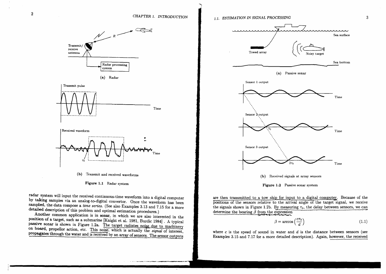
rameters. We briefly describe the first three of these systems. In radar we are mterested
in determining the position of an aircraft, as for example, in airport surveillance radar
[Skolnik 1980]. To determine the range R we transmit an electromagnetic pulse that is
the antenna To seconds later~
reflected by the aircraft, causin an echo to be received b
igure 1.1a. The range is determined by the equation TO = 2R/c, where
as shown in
c is the speed of electromagnetic propagation. Clearly, if the round trip delay To can
be measured, then so can the range. A typical transmit pulse and received waveform
a:e shown in Figure 1.1b. The received echo is decreased in amplitude due to propaga
tIon losses and hence may be obscured by environmental nois~. Its onset may also be
perturbed by time delays introduced by the electronics of the receiver. Determination
of the round trip delay can therefore require more than just a means of detecting a
jump in the power level at the receiver. It is important to note that a typical modern
l
�
2
CHAPTER 1. INTRODUCTION
1.1. ESTIMATION IN SIGNAL PROCESSING
3
Transmit/
receive
antenna
'-----+01 Radar processing
system
(a) Radar
Transmit pulse
....................... - - .................... - - ... -1
Time
Time
Received waveform
:---- -----_ ... -_ ... _-------,
TO
~--------- ... ------ .. -- __ ..!
(b) Transmit and received waveforms
Figure 1.1 Radar system
radar s!,stem will input the received continuous-time waveform into a digital computer
by takmg samples via an analog-to-digital convertor. Once the waveform has been
sampled, the data compose a time series. (See also Examples 3.13 and 7.15 for a more
detailed description of this problem and optimal estimation procedures.)
Another common application is in sonar, in which we are also interested in the
posi~ion of a target, such as a submarine [Knight et al. 1981, Burdic 1984] . A typical
passive sonar is shown in Figure 1.2a. The target radiates noise due to machiner:y
on board, propellor action, etc. This noise, which is actually the signal of interest,
propagates through the water and is received by an array of sensors. The sensor outputs
Towed array
Sea surface
Sea bottom
---------------~~---------------------------~
(a) Passive sonar
Sensor 1 output
~ Time
~'C7~ Time
Sensor 3 output
f ~ \~ /
Time
(b) Received signals at array sensors
Figure 1.2 Passive sonar system
are then transmitted to a tow ship for input to a digital computer. Because of the
positions of the sensors relative to the arrival angle of the target signal, we receive
the signals shown in Figure 1.2b. By measuring TO, the delay between sensors, we can
determine the bearing f3 Z
CHAPTER 1. INTRODUCTION
1.1. ESTIMATION IN SIGNAL PROCESSING
5
S :s
-.....
-.....
<0
.... .,
<0
u " C.
"' u. p.. -10
...:l
"'0 -20
<=
:d -30~
S
E
!
!?!' -40-+
!
-0
c -50 I
.;::
"
0
p..
S
::=..
301
-.....
'" 2°i
-.....
<0
t
10-+
u
::;
C.
0
-10
'" U
"-
...:l
"2 -20
id
~ -301
~ -40-+
~ -50il--------~I--------_r1 --------TI--------T-------~----
0::
1000
1500
2000
I
0
2500
500
Frequency (Hz)
Figure 1.4 LPC spectral modeling
4
-.....
-.....
<0
"&
.;,
:~
0
-1
-2
-3
0
2
4
6
8
10
12
Time (ms)
14
16
18
20
i
500
1000
1500
2000
Frequency (Hz)
I
2500
o
8
10
14
Time (ms)
Figure 1.3 Examples of speech sounds
waveforms are not "clean" as shown in Figure 1.2b but are embedded in noise, making,
the determination of To more difficult. The value of (3 obtained from (1.1) is then onli(
an estimate.
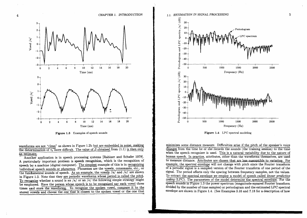
- Another application is in speech processing systems [Rabiner and Schafer 1978].
A particularly important problem is speech recognition, which is the recognition of
speech by a machine (digital computer). The simplest example of this is in recognizing
individual speech sounds or phonemes. Phonemes are the vowels, consonants, etc., or
the fundamental sounds of speech. As an example, the vowels /al and /e/ are shown
in Figure 1.3. Note that they are eriodic waveforms whose eriod is called the pitch.
To recognize whether a sound is an la or an lei the following simple strategy might
be employed. Have the person whose speech is to be recognized say each vowel three
times and store the waveforms. To reco nize the s oken vowel com are it to the
stored vowe s and choose the one that is closest to the spoken vowel or the one that
minimizes some distance measure. Difficulties arise if the
itch of the speaker's voice
c anges from the time he or s e recor s the sounds (the training session) to the time
when the speech recognizer is used. This is a natural variability due to the nature of
human speech. In practice, attributes, other than the waveforms themselves, are used
to measure distance. Attributes are chosen that are less sllsceptible to variation. For
example, the spectral envelope will not change with pitch since the Fourier transform
of a periodic signal is a sampled version of the Fourier transform of one period of the
signal. The period affects only the spacing between frequency samples, not the values.
To extract the s ectral envelo e we em 10 a model of s eech called linear predictive
coding LPC). The parameters of the model determine the s ectral envelope. For the
speec soun SIll 19ure 1.3 the power spectrum (magnitude-squared Fourier transform
divided by the number of time samples) or periodogram and the estimated LPC spectral
envelope are shown in Figure 1.4. (See Examples 3.16 and 7.18 for a description of how
�
6
CHAPTER 1.
INTRODUCTION
1.2. THE MATHEMATICAL ESTIMATION PROBLEM
7
x[O]
the parameters of the model are estimated and used to find the spectral envelope.) It
is interesting that in this example a human interpreter can easily discern the spoken
vowel. The real problem then is to design a machine that is able to do the same. In
the radar/sonar problem a human interpreter would be unable to determine the target
position from the received waveforms, so that the machine acts as an indispensable
tool.
In all these systems we are faced with the problem of extracting values of parameters
bas~ on continuous-time waveforms. Due to the use of di ital com uters to sample
and store
e contmuous-time wave orm, we have the equivalent problem of extractin
parameter values from a discrete-time waveform or a data set.
at ematically, we have
the N-point data set {x[O], x[I], ... , x[N -In which depends on an unknown parameter
(). We wish to determine () based on the data or to define an estimator
{J = g(x[O] , x[I], . .. , x[N - 1])
(1.2)
where 9 is some function. This is the problem of pammeter estimation, which is the
subject of this book. Although electrical engineers at one time designed systems based
on analog signals and analog circuits, the current and future trend is based on discrete
time signals or sequences and digital circuitry. With this transition the estimation
problem has evolved into one of estimating a parameter based on a time series, which
is just a discrete-time process. Furthermore, because the amount of data is necessarily
finite, we are faced with the determination of 9 as in (1.2). Therefore, our problem has
now evolved into one which has a long and glorious history, dating back to Gauss who
in 1795 used least squares data analysis to predict planetary m(Wements [Gauss 1963
(English translation)]. All the theory and techniques of statisti~al estimation are at
our disposal [Cox and Hinkley 1974, Kendall and Stuart 1976-1979, Rao 1973, Zacks
1981].
Before concluding our discussion of application areas we complete the previous list.
4. Image analysis - Elstimate the position and orientation of an object from a camera
image, necessary when using a robot to pick up an object [Jain 1989]
5. Biomedicine - estimate the heart rate of a fetu~ [Widrow and Stearns 1985]
6. Communications - estimate the carrier frequency of a signal so that the signal can
be demodulated to baseband [Proakis 1983]
1. Control - estimate the position of a powerboat so that corrective navigational
action can be taken, as in a LORAN system [Dabbous 1988]
8. Seismology - estimate the underground distance of an oil deposit based on SOUD&
reflections dueto the different densities of oil and rock layers [Justice 1985].
Finally, the multitude of applications stemming from analysis of data from physical
experiments, economics, etc., should also be mentioned [Box and Jenkins 1970, Holm
and Hovem 1979, Schuster 1898, Taylor 1986].
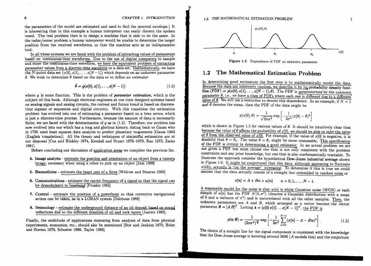
Figure 1.5 Dependence of PDF on unknown parameter
1.2 The Mathematical Estimation Problem
In determining good .estimators the first step is to mathematically model the data.
~ecause the data are mherently random, we describe it by it§, probability density func
tion (PDF) 01:" p(x[O], x[I], ... , x[N - 1]; ()). The PDF is parameterized by the unknown
l2arameter ()J I.e., we have a class of PDFs where each one is different due to a different
value of (). We will use a semicolon to denote this dependence. As an example, if N = 1
and () denotes the mean, then the PDF of the data might be
p(x[O]; ()) = .:-." exp [ __ I_(x[O] _ ())2]
v 27rO'2
20'2
which is shown in Figure 1.5 for various values of (). It should be intuitively clear that
because the value of () affects the probability of xiO], we should be able to infer the value
of () from the observed value of x[OL For example, if the value of x[O] is negative, it is
doubtful tha~ () =:' .()2' :rhe value. (). = ()l might be more reasonable, This specification
of th~ PDF IS cntlcal m determmmg a good estima~. In an actual problem we are
not glv~n a PDF but .must choose one that is not only consistent with the problem
~onstramts and any pnor knowledge, but one that is also mathematically tractable. To
~llus~rate the appr~ach consider the hypothetical Dow-Jones industrial average shown
IP. FIgure 1.6. It. mIght be conjectured that this data, although appearing to fluctuate
WIldly, actually IS "on the average" increasing. To determine if this is true we could
assume that the data actually consist of a straight line embedded in random noise or
x[n] =A+Bn+w[n]
n = 0, 1, ... ,N - 1.
~ reasonable model for the noise is that win] is white Gaussian noise (WGN) or each
sample of win] has the PDF N(0,O'2) (denotes a Gaussian distribution with a mean
of 0 and a variance of 0'2) and is uncorrelated with all the other samples. Then, the
unknown parameters are A and B, which arranged as a vector become the vector
parameter 9 = [A Bf. Letting x = [x[O] x[I] . .. x[N - lW, the PDF is
1
[1 N-l
p(x; 9) = (27rO'2)~ exp - 20'2 ~ (x[n]- A - Bn)2
.
(1.3)
]
The choice of a straight line for the signal component is consistent with the knowledge
that the Dow-Jones average is hovering around 3000 (A models this) and the conjecture
�



 2023年江西萍乡中考道德与法治真题及答案.doc
 2012年重庆南川中考生物真题及答案.doc
 2013年江西师范大学地理学综合及文艺理论基础考研真题.doc
 2020年四川甘孜小升初语文真题及答案I卷.doc
 2020年注册岩土工程师专业基础考试真题及答案.doc
 2023-2024学年福建省厦门市九年级上学期数学月考试题及答案.doc
 2021-2022学年辽宁省沈阳市大东区九年级上学期语文期末试题及答案.doc
 2022-2023学年北京东城区初三第一学期物理期末试卷及答案.doc
 2018上半年江西教师资格初中地理学科知识与教学能力真题及答案.doc
 2012年河北国家公务员申论考试真题及答案-省级.doc
 2020-2021学年江苏省扬州市江都区邵樊片九年级上学期数学第一次质量检测试题及答案.doc
 2022下半年黑龙江教师资格证中学综合素质真题及答案.doc