“GrabCut” — Interactive Foreground Extraction using Iterated Graph Cuts
Carsten Rother∗
Vladimir Kolmogorov†
Andrew Blake‡
Microsoft Research Cambridge, UK
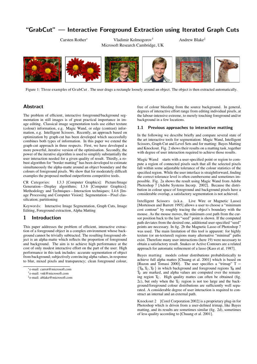
Figure 1: Three examples of GrabCut . The user drags a rectangle loosely around an object. The object is then extracted automatically.
Abstract
The problem of efficient, interactive foreground/background seg-
mentation in still images is of great practical importance in im-
age editing. Classical image segmentation tools use either texture
(colour) information, e.g. Magic Wand, or edge (contrast) infor-
mation, e.g. Intelligent Scissors. Recently, an approach based on
optimization by graph-cut has been developed which successfully
combines both types of information. In this paper we extend the
graph-cut approach in three respects. First, we have developed a
more powerful, iterative version of the optimisation. Secondly, the
power of the iterative algorithm is used to simplify substantially the
user interaction needed for a given quality of result. Thirdly, a ro-
bust algorithm for “border matting” has been developed to estimate
simultaneously the alpha-matte around an object boundary and the
colours of foreground pixels. We show that for moderately difficult
examples the proposed method outperforms competitive tools.
CR Categories:
I.3.3 [Computer Graphics]: Picture/Image
I.3.6 [Computer Graphics]:
Generation—Display algorithms;
Methodology and Techniques—Interaction techniques; I.4.6 [Im-
age Processing and Computer Vision]: Segmentation—Pixel clas-
sification; partitioning
Keywords:
Editing, Foreground extraction, Alpha Matting
Interactive Image Segmentation, Graph Cuts, Image
1
Introduction
This paper addresses the problem of efficient, interactive extrac-
tion of a foreground object in a complex environment whose back-
ground cannot be trivially subtracted. The resulting foreground ob-
ject is an alpha-matte which reflects the proportion of foreground
and background. The aim is to achieve high performance at the
cost of only modest interactive effort on the part of the user. High
performance in this task includes: accurate segmentation of object
from background; subjectively convincing alpha values, in response
to blur, mixed pixels and transparency; clean foreground colour,
∗e-mail: carrot@microsoft.com
†e-mail: vnk@microsoft.com
‡e-mail: ablake@microsoft.com
free of colour bleeding from the source background.
In general,
degrees of interactive effort range from editing individual pixels, at
the labour-intensive extreme, to merely touching foreground and/or
background in a few locations.
1.1 Previous approaches to interactive matting
In the following we describe briefly and compare several state of
the art interactive tools for segmentation: Magic Wand, Intelligent
Scissors, Graph Cut and Level Sets and for matting: Bayes Matting
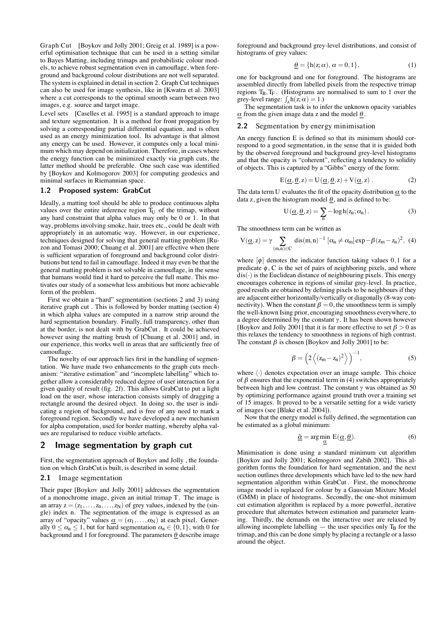
and Knockout. Fig. 2 shows their results on a matting task, together
with degree of user interaction required to achieve those results.
Magic Wand starts with a user-specified point or region to com-
pute a region of connected pixels such that all the selected pixels
fall within some adjustable tolerance of the colour statistics of the
specified region. While the user interface is straightforward, finding
the correct tolerance level is often cumbersome and sometimes im-
possible. Fig. 2a shows the result using Magic Wand from Adobe
Photoshop 7 [Adobe Systems Incorp. 2002]. Because the distri-
bution in colour space of foreground and background pixels have a
considerable overlap, a satisfactory segmentation is not achieved.
(a.k.a.
Intelligent Scissors
Live Wire or Magnetic Lasso)
[Mortensen and Barrett 1995] allows a user to choose a “minimum
cost contour” by roughly tracing the object’s boundary with the
mouse. As the mouse moves, the minimum cost path from the cur-
sor position back to the last “seed” point is shown. If the computed
path deviates from the desired one, additional user-specified “seed”
points are necessary. In fig. 2b the Magnetic Lasso of Photoshop 7
was used. The main limitation of this tool is apparent: for highly
texture (or un-textured) regions many alternative “minimal” paths
exist. Therefore many user interactions (here 19) were necessary to
obtain a satisfactory result. Snakes or Active Contours are a related
approach for automatic refinement of a lasso [Kass et al. 1987].
Bayes matting models colour distributions probabilistically to
achieve full alpha mattes [Chuang et al. 2001] which is based on
[Ruzon and Tomasi 2000]. The user specifies a “trimap” T =
{TB, TU , TF } in which background and foreground regions TB and
TF are marked, and alpha values are computed over the remain-
ing region TU . High quality mattes can often be obtained (fig.
2c), but only when the TU region is not too large and the back-
ground/foreground colour distributions are sufficiently well sepa-
rated. A considerable degree of user interaction is required to con-
struct an internal and an external path.
Knockout 2 [Corel Corporation 2002] is a proprietary plug-in for
Photoshop which is driven from a user-defined trimap, like Bayes
matting, and its results are sometimes similar (fig. 2d), sometimes
of less quality according to [Chuang et al. 2001].
�
Graph Cut
[Boykov and Jolly 2001; Greig et al. 1989] is a pow-
erful optimisation technique that can be used in a setting similar
to Bayes Matting, including trimaps and probabilistic colour mod-
els, to achieve robust segmentation even in camouflage, when fore-
ground and background colour distributions are not well separated.
The system is explained in detail in section 2. Graph Cut techniques
can also be used for image synthesis, like in [Kwatra et al. 2003]
where a cut corresponds to the optimal smooth seam between two
images, e.g. source and target image.
Level sets
[Caselles et al. 1995] is a standard approach to image
and texture segmentation. It is a method for front propagation by
solving a corresponding partial differential equation, and is often
used as an energy minimization tool. Its advantage is that almost
any energy can be used. However, it computes only a local mini-
mum which may depend on initialization. Therefore, in cases where
the energy function can be minimized exactly via graph cuts, the
latter method should be preferable. One such case was identified
by [Boykov and Kolmogorov 2003] for computing geodesics and
minimal surfaces in Riemannian space.
1.2 Proposed system: GrabCut
Ideally, a matting tool should be able to produce continuous alpha
values over the entire inference region TU of the trimap, without
any hard constraint that alpha values may only be 0 or 1. In that
way, problems involving smoke, hair, trees etc., could be dealt with
appropriately in an automatic way. However, in our experience,
techniques designed for solving that general matting problem [Ru-
zon and Tomasi 2000; Chuang et al. 2001] are effective when there
is sufficient separation of foreground and background color distri-
butions but tend to fail in camouflage. Indeed it may even be that the
general matting problem is not solvable in camouflage, in the sense
that humans would find it hard to perceive the full matte. This mo-
tivates our study of a somewhat less ambitious but more achievable
form of the problem.
First we obtain a “hard” segmentation (sections 2 and 3) using
iterative graph cut . This is followed by border matting (section 4)
in which alpha values are computed in a narrow strip around the
hard segmentation boundary. Finally, full transparency, other than
at the border, is not dealt with by GrabCut . It could be achieved
however using the matting brush of [Chuang et al. 2001] and, in
our experience, this works well in areas that are sufficiently free of
camouflage.
The novelty of our approach lies first in the handling of segmen-
tation. We have made two enhancements to the graph cuts mech-
anism: “iterative estimation” and “incomplete labelling” which to-
gether allow a considerably reduced degree of user interaction for a
given quality of result (fig. 2f). This allows GrabCut to put a light
load on the user, whose interaction consists simply of dragging a
rectangle around the desired object. In doing so, the user is indi-
cating a region of background, and is free of any need to mark a
foreground region. Secondly we have developed a new mechanism
for alpha computation, used for border matting, whereby alpha val-
ues are regularised to reduce visible artefacts.
2
Image segmentation by graph cut
First, the segmentation approach of Boykov and Jolly , the founda-
tion on which GrabCut is built, is described in some detail.
2.1
Image segmentation
Their paper [Boykov and Jolly 2001] addresses the segmentation
of a monochrome image, given an initial trimap T . The image is
an array z = (z1, . . . , zn, . . . , zN ) of grey values, indexed by the (sin-
gle) index n. The segmentation of the image is expressed as an
array of “opacity” values a = (a 1, . . . ,a N ) at each pixel. Gener-
ally 0 ≤ a n ≤ 1, but for hard segmentation a n ∈ {0,1}, with 0 for
background and 1 for foreground. The parameters q describe image
foreground and background grey-level distributions, and consist of
histograms of grey values:
q = {h(z;a ), a = 0,1},
(1)
one for background and one for foreground. The histograms are
assembled directly from labelled pixels from the respective trimap
regions TB, TF . (Histograms are normalised to sum to 1 over the
grey-level range: Rz h(z;a ) = 1.)
The segmentation task is to infer the unknown opacity variables
a
from the given image data z and the model q .
2.2 Segmentation by energy minimisation
An energy function E is defined so that its minimum should cor-
respond to a good segmentation, in the sense that it is guided both
by the observed foreground and background grey-level histograms
and that the opacity is “coherent”, reflecting a tendency to solidity
of objects. This is captured by a “Gibbs” energy of the form:
E(a ,q ,z) = U(a ,q ,z) +V (a ,z) .
The data term U evaluates the fit of the opacity distribution a
data z, given the histogram model q , and is defined to be:
U(a ,q ,z) =
−log h(zn;a n) .
n
(2)
to the
(3)
The smoothness term can be written as
V (a ,z) = g
dis(m, n)−1 [a n 6= a m]exp −b (zm − zn)2, (4)
(m,n)∈C
where [f ] denotes the indicator function taking values 0,1 for a
predicate f , C is the set of pairs of neighboring pixels, and where
dis(·) is the Euclidean distance of neighbouring pixels. This energy
encourages coherence in regions of similar grey-level. In practice,
good results are obtained by defining pixels to be neighbours if they
are adjacent either horizontally/vertically or diagonally (8-way con-
nectivity). When the constant b = 0, the smoothness term is simply
the well-known Ising prior, encouraging smoothness everywhere, to
a degree determined by the constant g . It has been shown however
[Boykov and Jolly 2001] that it is far more effective to set b > 0 as
this relaxes the tendency to smoothness in regions of high contrast.
The constant b
is chosen [Boykov and Jolly 2001] to be:
b = 2D(zm − zn)2E−1
,
(5)
where h·i denotes expectation over an image sample. This choice
of b ensures that the exponential term in (4) switches appropriately
between high and low contrast. The constant g was obtained as 50
by optimizing performance against ground truth over a training set
of 15 images. It proved to be a versatile setting for a wide variety
of images (see [Blake et al. 2004]).
Now that the energy model is fully defined, the segmentation can
be estimated as a global minimum:
ˆa = argmina E(a ,q ).
(6)
Minimisation is done using a standard minimum cut algorithm
[Boykov and Jolly 2001; Kolmogorov and Zabih 2002]. This al-
gorithm forms the foundation for hard segmentation, and the next
section outlines three developments which have led to the new hard
segmentation algorithm within GrabCut . First, the monochrome
image model is replaced for colour by a Gaussian Mixture Model
(GMM) in place of histograms. Secondly, the one-shot minimum
cut estimation algorithm is replaced by a more powerful, iterative
procedure that alternates between estimation and parameter learn-
ing. Thirdly, the demands on the interactive user are relaxed by
allowing incomplete labelling — the user specifies only TB for the
trimap, and this can be done simply by placing a rectangle or a lasso
around the object.
�
Magic Wand
Intelligent Scissors
Bayes Matte
Knockout 2
Graph cut
GrabCut
(a)
(b)
(c)
(d)
(e)
(f)
Figure 2: Comparison of some matting and segmentation tools. The top row shows the user interaction required to complete the segmenta-
tion or matting process: white brush/lasso (foreground), red brush/lasso (background), yellow crosses (boundary). The bottom row illustrates
the resulting segmentation. GrabCut appears to outperform the other approaches both in terms of the simplicity of user input and the quality
of results. Original images on the top row are displayed with reduced intensity to facilitate overlay; see fig. 1. for original. Note that our
implementation of Graph Cut [Boykov and Jolly 2001] uses colour mixture models instead of grey value histograms.
3 The GrabCut segmentation algorithm
This section describes the novel parts of the GrabCut hard segmen-
tation algorithm: iterative estimation and incomplete labelling.
3.1 Colour data modelling
The image is now taken to consist of pixels zn in RGB colour space.
As it is impractical to construct adequate colour space histograms,
we follow a practice that is already used for soft segmentation [Ru-
zon and Tomasi 2000; Chuang et al. 2001] and use GMMs. Each
GMM, one for the background and one for the foreground, is taken
to be a full-covariance Gaussian mixture with K components (typi-
cally K = 5). In order to deal with the GMM tractably, in the opti-
mization framework, an additional vector k = {k1, . . . , kn, . . . , kN } is
introduced, with kn ∈ {1, . . .K}, assigning, to each pixel, a unique
GMM component, one component either from the background or
the foreground model, according as a n = 0 or 11.
The Gibbs energy (2) for segmentation now becomes
E(a ,k,q ,z) = U(a ,k,q ,z) +V (a ,z),
(7)
depending also on the GMM component variables k. The data term
U is now defined, taking account of the colour GMM models, as
U(a ,k,q ,z) =
D(a n, kn,q , zn),
n
(8)
where D(a n, kn,q , zn) = −log p(zn | a n, kn,q ) − logp (a n, kn), and
p(·) is a Gaussian probability distribution, and p (·) are mixture
weighting coefficients, so that (up to a constant):
D(a n, kn,q , zn) = −logp (a n, kn) +
logdetS (a n, kn)
(9)
1
2
+
1
2
[zn − m (a n, kn)]>S (a n, kn)−1[zn − m (a n, kn)].
Therefore, the parameters of the model are now
q = {p (a , k), m (a , k),S (a , k), a = 0,1, k = 1 . . .K} ,
(10)
1Soft assignments of probabilities for each component to a given pixel
might seem preferable as it would allow “Expectation Maximization”
[Dempster et al. 1977] to be used; however that involves significant addi-
tional computational expense for what turns out to be negligible practical
benefit.
i.e. the weights p , means m and covariances S of the 2K Gaussian
components for the background and foreground distributions. The
smoothness term V is basically unchanged from the monochrome
case (4) except that the contrast term is computed using Euclidean
distance in colour space:
V (a ,z) = g
[a n 6= a m]exp −b kzm − znk2 .
(11)
(m,n)∈C
3.2 Segmentation by iterative energy minimization
The new energy minimization scheme in GrabCut works iteratively,
in place of the previous one-shot algorithm [Boykov and Jolly
2001]. This has the advantage of allowing automatic refinement
of the opacities a , as newly labelled pixels from the TU region of
the initial trimap are used to refine the colour GMM parameters
q . The main elements of the GrabCut system are given in fig. 3.
Step 1 is straightforward, done by simple enumeration of the kn
values for each pixel n. Step 2 is implemented as a set of Gaussian
parameter estimation procedures, as follows. For a given GMM
component k in, say, the foreground model, the subset of pixels
F(k) = {zn : kn = k and a n = 1} is defined. The mean m (a , k) and
covariance S (a , k) are estimated in standard fashion as the sam-
ple mean and covariance of pixel values in F(k) and weights are
p (a , k) = |F(k)|/
k |F(k)|, where |S| denotes the size of a set S.
Finally step 3 is a global optimization, using minimum cut, exactly
as [Boykov and Jolly 2001].
The structure of the algorithm guarantees proper convergence
properties. This is because each of steps 1 to 3 of iterative min-
imisation can be shown to be a minimisation of the total energy E
with respect to the three sets of variables k, q , a
in turn. Hence
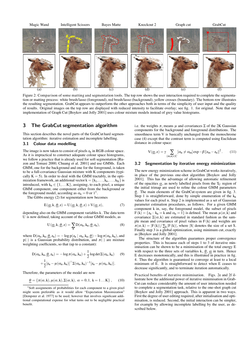
E decreases monotonically, and this is illustrated in practice in fig.
4. Thus the algorithm is guaranteed to converge at least to a local
minimum of E.
It is straightforward to detect when E ceases to
decrease significantly, and to terminate iteration automatically.
Practical benefits of iterative minimisation. Figs. 2e and 2f il-
lustrate how the additional power of iterative minimisation in Grab-
Cut can reduce considerably the amount of user interaction needed
to complete a segmentation task, relative to the one-shot graph cut
[Boykov and Jolly 2001] approach. This is apparent in two ways.
First the degree of user editing required, after initialisation and opti-
misation, is reduced. Second, the initial interaction can be simpler,
for example by allowing incomplete labelling by the user, as de-
scribed below.
�
Initialisation
• User initialises trimap T by supplying only TB. The fore-
ground is set to TF = /0; TU = T B, complement of the back-
ground.
• Initialise a n = 0 for n ∈ TB and a n = 1 for n ∈ TU .
• Background and foreground GMMs initialised from sets
a n = 0 and a n = 1 respectively.
Iterative minimisation
1. Assign GMM components to pixels: for each n in TU ,
kn := argmin
kn
Dn(a n, kn,q , zn).
2. Learn GMM parameters from data z:
q
:= argminq U(a ,k,q ,z)
3. Estimate segmentation: use min cut to solve:
min
{a n: n∈TU }
min
k
E(a ,k,q ,z).
4. Repeat from step 1, until convergence.
5. Apply border matting (section 4).
User editing
• Edit: fix some pixels either to a n = 0 (background brush)
or a n = 1 (foreground brush); update trimap T accord-
ingly. Perform step 3 above, just once.
• Refine operation: [optional] perform entire iterative min-
imisation algorithm.
Figure 3: Iterative image segmentation in GrabCut
Energy E
N
E
E
R
G
N
E
E
R
G
1
4
8
12
(a)
RED
(b)
RED
(c)
Figure 4: Convergence of iterative minimization for the data of
fig. 2f. (a) The energy E for the llama example converges over
12 iterations. The GMM in RGB colour space (side-view showing
R,G) at initialization (b) and after convergence (c). K = 5 mixture
components were used for both background (red) and foreground
(blue). Initially (b) both GMMs overlap considerably, but are bet-
ter separated after convergence (c), as the foreground/background
labelling has become accurate.
3.3 User Interaction and incomplete trimaps
Incomplete trimaps. The iterative minimisation algorithm al-
lows increased versatility of user interaction. In particular, incom-
plete labelling becomes feasible where, in place of the full trimap
T , the user needs only specify, say, the background region TB, leav-
ing TF = 0. No hard foreground labelling is done at all. Iterative
minimisation (fig. 3) deals with this incompleteness by allowing
provisional labels on some pixels (in the foreground) which can
subsequently be retracted; only the background labels TB are taken
to be firm — guaranteed not to be retracted later. (Of course a com-
plementary scheme, with firm labels for the foreground only, is also
a possibility.) In our implementation, the initial TB is determined by
the user as a strip of pixels around the outside of the marked rect-
angle (marked in red in fig. 2f).
Automatic
Segmentation
U s e r
I n t e r a c t i o n
Automatic
Segmentation
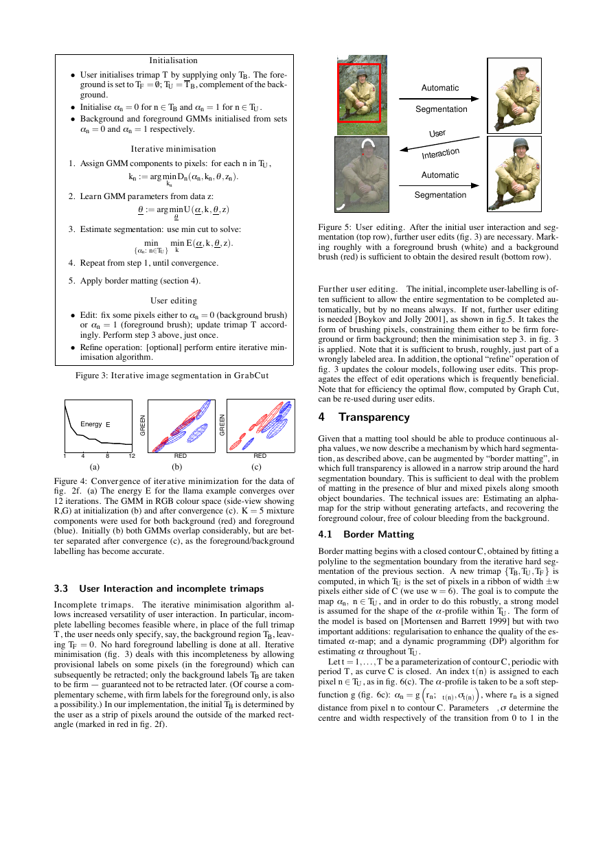
Figure 5: User editing. After the initial user interaction and seg-
mentation (top row), further user edits (fig. 3) are necessary. Mark-
ing roughly with a foreground brush (white) and a background
brush (red) is sufficient to obtain the desired result (bottom row).
Further user editing. The initial, incomplete user-labelling is of-
ten sufficient to allow the entire segmentation to be completed au-
tomatically, but by no means always. If not, further user editing
is needed [Boykov and Jolly 2001], as shown in fig.5. It takes the
form of brushing pixels, constraining them either to be firm fore-
ground or firm background; then the minimisation step 3. in fig. 3
is applied. Note that it is sufficient to brush, roughly, just part of a
wrongly labeled area. In addition, the optional “refine” operation of
fig. 3 updates the colour models, following user edits. This prop-
agates the effect of edit operations which is frequently beneficial.
Note that for efficiency the optimal flow, computed by Graph Cut,
can be re-used during user edits.
4 Transparency
Given that a matting tool should be able to produce continuous al-
pha values, we now describe a mechanism by which hard segmenta-
tion, as described above, can be augmented by “border matting”, in
which full transparency is allowed in a narrow strip around the hard
segmentation boundary. This is sufficient to deal with the problem
of matting in the presence of blur and mixed pixels along smooth
object boundaries. The technical issues are: Estimating an alpha-
map for the strip without generating artefacts, and recovering the
foreground colour, free of colour bleeding from the background.
4.1 Border Matting
Border matting begins with a closed contour C, obtained by fitting a
polyline to the segmentation boundary from the iterative hard seg-
mentation of the previous section. A new trimap {TB, TU , TF } is
computed, in which TU is the set of pixels in a ribbon of width ±w
pixels either side of C (we use w = 6). The goal is to compute the
map a n, n ∈ TU , and in order to do this robustly, a strong model
is assumed for the shape of the a -profile within TU . The form of
the model is based on [Mortensen and Barrett 1999] but with two
important additions: regularisation to enhance the quality of the es-
timated a -map; and a dynamic programming (DP) algorithm for
estimating a
throughout TU .
Let t = 1, . . . , T be a parameterization of contour C, periodic with
period T , as curve C is closed. An index t(n) is assigned to each
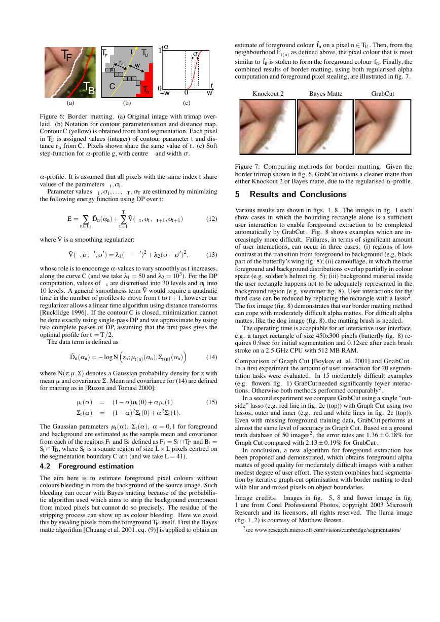
pixel n ∈ TU , as in fig. 6(c). The a -profile is taken to be a soft step-
function g (fig. 6c): a n = grn;D
t(n),s t(n), where rn is a signed
distance from pixel n to contour C. Parameters D
,s determine the
centre and width respectively of the transition from 0 to 1 in the
�
T
F
F T
n
C
T
B
(a)
(b)
a
1
s
t
U T
w
r
n
B T
0
−w
r
w
D 0
(c)
Figure 6: Border matting. (a) Original image with trimap over-
laid. (b) Notation for contour parameterisation and distance map.
Contour C (yellow) is obtained from hard segmentation. Each pixel
in TU is assigned values (integer) of contour parameter t and dis-
tance rn from C. Pixels shown share the same value of t. (c) Soft
step-function for a -profile g, with centre D and width s .
a -profile. It is assumed that all pixels with the same index t share
values of the parameters D
Parameter values D 1,s 1, . . . ,D T ,s T are estimated by minimizing
t ,s t.
the following energy function using DP over t:
E =
˜Dn(a n) +
n∈TU
T
t=1
˜V (D
t ,s t ,D
t+1,s t+1)
(12)
0)2 + l 2(s − s
0)2,
where ˜V is a smoothing regularizer:
0) = l 1(D − D
,s ,D
˜V (D
0,s
(13)
whose role is to encourage a -values to vary smoothly as t increases,
along the curve C (and we take l 1 = 50 and l 2 = 103). For the DP
t are discretised into 30 levels and s t into
computation, values of D
10 levels. A general smoothness term ˜V would require a quadratic
time in the number of profiles to move from t to t + 1, however our
regularizer allows a linear time algorithm using distance transforms
[Rucklidge 1996]. If the contour C is closed, minimization cannot
be done exactly using single-pass DP and we approximate by using
two complete passes of DP, assuming that the first pass gives the
optimal profile for t = T /2.
The data term is defined as
˜Dn(a n) = −logNzn; m t(n)(a n),S
t(n)(a n)
(14)
where N(z; m ,S ) denotes a Gaussian probability density for z with
mean m and covariance S
. Mean and covariance for (14) are defined
for matting as in [Ruzon and Tomasi 2000]:
m t (a ) = (1 − a )m t (0) + am
t (0) + a 2S
t (a ) = (1 − a )2S
t (a ), a = 0,1 for foreground
The Gaussian parameters m t (a ), S
and background are estimated as the sample mean and covariance
from each of the regions Ft and Bt defined as Ft = St ∩ TF and Bt =
St ∩ TB, where St is a square region of size L × L pixels centred on
the segmentation boundary C at t (and we take L = 41).
4.2 Foreground estimation
t (1).
t (1)
(15)
The aim here is to estimate foreground pixel colours without
colours bleeding in from the background of the source image. Such
bleeding can occur with Bayes matting because of the probabilis-
tic algorithm used which aims to strip the background component
from mixed pixels but cannot do so precisely. The residue of the
stripping process can show up as colour bleeding. Here we avoid
this by stealing pixels from the foreground TF itself. First the Bayes
matte algorithm [Chuang et al. 2001, eq. (9)] is applied to obtain an
estimate of foreground colour ˆfn on a pixel n ∈ TU . Then, from the
neighbourhood Ft(n) as defined above, the pixel colour that is most
similar to ˆfn is stolen to form the foreground colour fn. Finally, the
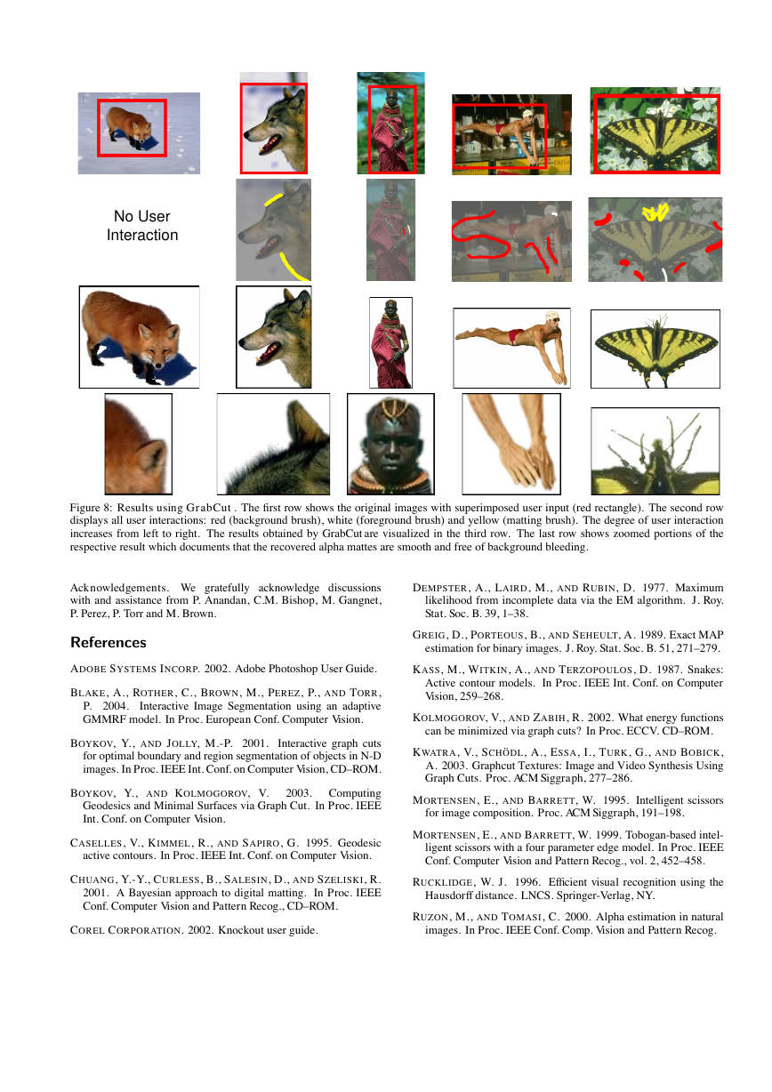
combined results of border matting, using both regularised alpha
computation and foreground pixel stealing, are illustrated in fig. 7.
Knockout 2
Bayes Matte
GrabCut
Figure 7: Comparing methods for border matting. Given the
border trimap shown in fig. 6, GrabCut obtains a cleaner matte than
either Knockout 2 or Bayes matte, due to the regularised a -profile.
5 Results and Conclusions
Various results are shown in figs. 1, 8. The images in fig. 1 each
show cases in which the bounding rectangle alone is a sufficient
user interaction to enable foreground extraction to be completed
automatically by GrabCut . Fig. 8 shows examples which are in-
creasingly more difficult. Failures, in terms of significant amount
of user interactions, can occur in three cases: (i) regions of low
contrast at the transition from foreground to background (e.g. black
part of the butterfly’s wing fig. 8); (ii) camouflage, in which the true
foreground and background distributions overlap partially in colour
space (e.g. soldier’s helmet fig. 5); (iii) background material inside
the user rectangle happens not to be adequately represented in the
background region (e.g. swimmer fig. 8). User interactions for the
third case can be reduced by replacing the rectangle with a lasso2.
The fox image (fig. 8) demonstrates that our border matting method
can cope with moderately difficult alpha mattes. For difficult alpha
mattes, like the dog image (fig. 8), the matting brush is needed.
The operating time is acceptable for an interactive user interface,
e.g. a target rectangle of size 450x300 pixels (butterfly fig. 8) re-
quires 0.9sec for initial segmentation and 0.12sec after each brush
stroke on a 2.5 GHz CPU with 512 MB RAM.
Comparison of Graph Cut [Boykov et. al. 2001] and GrabCut .
In a first experiment the amount of user interaction for 20 segmen-
tation tasks were evaluated.
In 15 moderately difficult examples
(e.g. flowers fig. 1) GrabCut needed significantly fewer interac-
tions. Otherwise both methods performed comparably2.
In a second experiment we compare GrabCut using a single “out-
side” lasso (e.g. red line in fig. 2c (top)) with Graph Cut using two
lassos, outer and inner (e.g. red and white lines in fig. 2c (top)).
Even with missing foreground training data, GrabCut performs at
almost the same level of accuracy as Graph Cut. Based on a ground
truth database of 50 images2, the error rates are 1.36 ± 0.18% for
Graph Cut compared with 2.13 ± 0.19% for GrabCut .
In conclusion, a new algorithm for foreground extraction has
been proposed and demonstrated, which obtains foreground alpha
mattes of good quality for moderately difficult images with a rather
modest degree of user effort. The system combines hard segmenta-
tion by iterative graph-cut optimisation with border matting to deal
with blur and mixed pixels on object boundaries.
Image credits.
Images in fig. 5, 8 and flower image in fig.
1 are from Corel Professional Photos, copyright 2003 Microsoft
Research and its licensors, all rights reserved. The llama image
(fig. 1, 2) is courtesy of Matthew Brown.
2see www.research.microsoft.com/vision/cambridge/segmentation/
S
�
No User
Interaction
Figure 8: Results using GrabCut . The first row shows the original images with superimposed user input (red rectangle). The second row
displays all user interactions: red (background brush), white (foreground brush) and yellow (matting brush). The degree of user interaction
increases from left to right. The results obtained by GrabCut are visualized in the third row. The last row shows zoomed portions of the
respective result which documents that the recovered alpha mattes are smooth and free of background bleeding.
Acknowledgements. We gratefully acknowledge discussions
with and assistance from P. Anandan, C.M. Bishop, M. Gangnet,
P. Perez, P. Torr and M. Brown.
DEMPSTER, A., LAIRD, M., AND RUBIN, D. 1977. Maximum
likelihood from incomplete data via the EM algorithm. J. Roy.
Stat. Soc. B. 39, 1–38.
References
ADOBE SYSTEMS INCORP. 2002. Adobe Photoshop User Guide.
BLAKE, A., ROTHER, C., BROWN, M., PEREZ, P., AND TORR,
Interactive Image Segmentation using an adaptive
P. 2004.
GMMRF model. In Proc. European Conf. Computer Vision.
BOYKOV, Y., AND JOLLY, M.-P. 2001.
Interactive graph cuts
for optimal boundary and region segmentation of objects in N-D
images. In Proc. IEEE Int. Conf. on Computer Vision, CD–ROM.
BOYKOV, Y., AND KOLMOGOROV, V.
Computing
Geodesics and Minimal Surfaces via Graph Cut. In Proc. IEEE
Int. Conf. on Computer Vision.
2003.
CASELLES, V., KIMMEL, R., AND SAPIRO, G. 1995. Geodesic
active contours. In Proc. IEEE Int. Conf. on Computer Vision.
CHUANG, Y.-Y., CURLESS, B., SALESIN, D., AND SZELISKI, R.
2001. A Bayesian approach to digital matting. In Proc. IEEE
Conf. Computer Vision and Pattern Recog., CD–ROM.
COREL CORPORATION. 2002. Knockout user guide.
GREIG, D., PORTEOUS, B., AND SEHEULT, A. 1989. Exact MAP
estimation for binary images. J. Roy. Stat. Soc. B. 51, 271–279.
KASS, M., WITKIN, A., AND TERZOPOULOS, D. 1987. Snakes:
Active contour models. In Proc. IEEE Int. Conf. on Computer
Vision, 259–268.
KOLMOGOROV, V., AND ZABIH, R. 2002. What energy functions
can be minimized via graph cuts? In Proc. ECCV. CD–ROM.
KWATRA, V., SCH ¨ODL, A., ESSA, I., TURK, G., AND BOBICK,
A. 2003. Graphcut Textures: Image and Video Synthesis Using
Graph Cuts. Proc. ACM Siggraph, 277–286.
MORTENSEN, E., AND BARRETT, W. 1995. Intelligent scissors
for image composition. Proc. ACM Siggraph, 191–198.
MORTENSEN, E., AND BARRETT, W. 1999. Tobogan-based intel-
ligent scissors with a four parameter edge model. In Proc. IEEE
Conf. Computer Vision and Pattern Recog., vol. 2, 452–458.
RUCKLIDGE, W. J. 1996. Efficient visual recognition using the
Hausdorff distance. LNCS. Springer-Verlag, NY.
RUZON, M., AND TOMASI, C. 2000. Alpha estimation in natural
images. In Proc. IEEE Conf. Comp. Vision and Pattern Recog.
�


 2023年江西萍乡中考道德与法治真题及答案.doc
 2012年重庆南川中考生物真题及答案.doc
 2013年江西师范大学地理学综合及文艺理论基础考研真题.doc
 2020年四川甘孜小升初语文真题及答案I卷.doc
 2020年注册岩土工程师专业基础考试真题及答案.doc
 2023-2024学年福建省厦门市九年级上学期数学月考试题及答案.doc
 2021-2022学年辽宁省沈阳市大东区九年级上学期语文期末试题及答案.doc
 2022-2023学年北京东城区初三第一学期物理期末试卷及答案.doc
 2018上半年江西教师资格初中地理学科知识与教学能力真题及答案.doc
 2012年河北国家公务员申论考试真题及答案-省级.doc
 2020-2021学年江苏省扬州市江都区邵樊片九年级上学期数学第一次质量检测试题及答案.doc
 2022下半年黑龙江教师资格证中学综合素质真题及答案.doc