正态分布乘积等于正态分布的证明.pdf

发布时间：2022-06-13 发布人：admin 分类：说明书资料大小：0.17M 资料格式：pdf 举报版权申诉

0e719f6c-2875-411c-baa8-021d8722d200.pdf-第1页.png

第1页 / 共13页

0e719f6c-2875-411c-baa8-021d8722d200.pdf-第2页.png

第2页 / 共13页

0e719f6c-2875-411c-baa8-021d8722d200.pdf-第3页.png

第3页 / 共13页

0e719f6c-2875-411c-baa8-021d8722d200.pdf-第4页.png

第4页 / 共13页

0e719f6c-2875-411c-baa8-021d8722d200.pdf-第5页.png

第5页 / 共13页

0e719f6c-2875-411c-baa8-021d8722d200.pdf-第6页.png

第6页 / 共13页

0e719f6c-2875-411c-baa8-021d8722d200.pdf-第7页.png

第7页 / 共13页

0e719f6c-2875-411c-baa8-021d8722d200.pdf-第8页.png

第8页 / 共13页

文本预览

Tina Memo No. 2003-003 Internal Report Products and Convolutions of Gaussian Probability Density Functions P.A. Bromiley Last updated 14 / 8 / 2014 Imaging Sciences Research Group, Institute of Population Health, School of Medicine, University of Manchester, Stopford Building, Oxford Road, Manchester, M13 9PT.

Products and Convolutions of Gaussian Probability Density Functions Imaging Sciences Research Group, Institute of Population Health, School of Medicine, University of Manchester, P. A. Bromiley Manchester, M13 9PT, UK paul.bromiley@manchester.ac.uk Abstract It is well known that the product and the convolution of Gaussian probability density functions (PDFs) are also Gaussian functions. This document provides proofs of this for several cases; the product of two univariate Gaussian PDFs, the product of an arbitrary number of univariate Gaussian PDFs, the product of an arbitrary number of multivariate Gaussian PDFs, and the convolution of two univari- ate Gaussian PDFs. These results are useful in calculating the eﬀects of smoothing applied as an intermediate step in various algorithms. 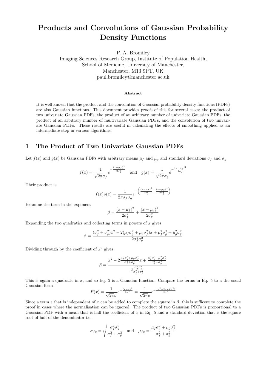1 The Product of Two Univariate Gaussian PDFs Let f (x) and g(x) be Gaussian PDFs with arbitrary means µf and µg and standard deviations σf and σg f (x) = 1 √2πσf − e (x−µf )2 2σ2 f and g(x) = (x−µg )2 2σ2 g 1 √2πσg − e Their product is Examine the term in the exponent f (x)g(x) = − (x−µf )2 2σ2 f + e 1 2πσf σg (x−µg )2 g 2σ2 β = (x − µf )2 2σ2 f + (x − µg)2 2σ2 g Expanding the two quadratics and collecting terms in powers of x gives (σ2 f + σ2 g)x2 − 2(µf σ2 β = g + µgσ2 2σ2 f σ2 g f )x + µ2 f σ2 g + µ2 gσ2 f Dividing through by the coeﬃcient of x2 gives x2 − 2 β = gσ2 f g+µ2 f σ2 µ2 σ2 f +σ2 g g+µgσ2 µf σ2 σ2 f +σ2 f x + g σ2 f σ2 σ2 f +σ2 g g 2 This is again a quadratic in x, and so Eq. 2 is a Gaussian function. Compare the terms in Eq. 5 to a the usual Gaussian form P (x) = 1 √2πσ e− (x−µ)2 2σ2 = 1 √2πσ e− (x2−2µx+µ2 ) 2σ2 Since a term ǫ that is independent of x can be added to complete the square in β, this is suﬃcent to complete the proof in cases where the normalisation can be ignored. The product of two Gaussian PDFs is proportional to a Gaussian PDF with a mean that is half the coeﬃcient of x in Eq. 5 and a standard deviation that is the square root of half of the denominator i.e. σf g =s σ2 f σ2 g σ2 f + σ2 g and µf g = g + µgσ2 µf σ2 f σ2 f + σ2 g

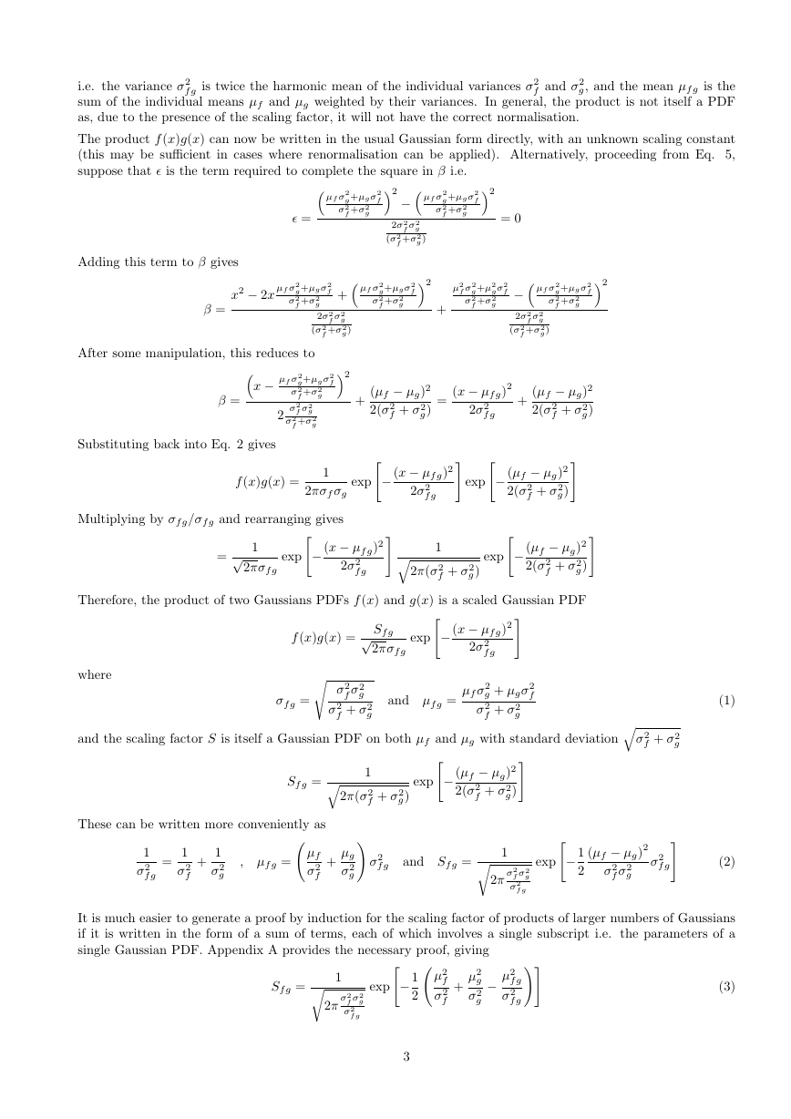
i.e. the variance σ2 g, and the mean µf g is the sum of the individual means µf and µg weighted by their variances. In general, the product is not itself a PDF as, due to the presence of the scaling factor, it will not have the correct normalisation. f g is twice the harmonic mean of the individual variances σ2 f and σ2 The product f (x)g(x) can now be written in the usual Gaussian form directly, with an unknown scaling constant (this may be suﬃcient in cases where renormalisation can be applied). Alternatively, proceeding from Eq. 5, suppose that ǫ is the term required to complete the square in β i.e. ǫ = µf σ2 g+µgσ2 σ2 f +σ2 f g 2 − µf σ2 g+µgσ2 σ2 f +σ2 f g 2 2σ2 f σ2 g f +σ2 g) (σ2 = 0 Adding this term to β gives x2 − 2x β = g+µgσ2 µf σ2 σ2 f +σ2 f + µf σ2 g+µgσ2 σ2 f +σ2 f g 2 g 2σ2 f σ2 g f +σ2 g) (σ2 + g+µ2 f σ2 µ2 σ2 f +σ2 f gσ2 g − µf σ2 2σ2 f σ2 g f +σ2 g) (σ2 g+µgσ2 σ2 f +σ2 f g 2 After some manipulation, this reduces to β = x − Substituting back into Eq. 2 gives f g 2 µf σ2 g+µgσ2 σ2 f +σ2 σ2 f σ2 σ2 f +σ2 g g 2 + (µf − µg)2 2(σ2 f + σ2 g) = (x − µf g)2 2σ2 f g + (µf − µg)2 2(σ2 f + σ2 g) f (x)g(x) = 1 2πσf σg exp"− (x − µf g)2 2σ2 f g # exp"− g)# (µf − µg)2 2(σ2 f + σ2 Multiplying by σf g/σf g and rearranging gives = 1 √2πσf g exp"− (x − µf g)2 2σ2 f g # exp"− g)# (µf − µg)2 2(σ2 f + σ2 f + σ2 g) Therefore, the product of two Gaussians PDFs f (x) and g(x) is a scaled Gaussian PDF 1 q2π(σ2 exp"− f (x)g(x) = Sf g√2πσf g (x − µf g)2 2σ2 f g # where σf g =s σ2 f σ2 g σ2 f + σ2 g and µf g = µf σ2 g + µgσ2 f σ2 f + σ2 g (1) and the scaling factor S is itself a Gaussian PDF on both µf and µg with standard deviation qσ2 f + σ2 g Sf g = These can be written more conveniently as 1 σ2 f g = 1 σ2 f + 1 σ2 g , µf g = µf σ2 f q2π(σ2 g! σ2 µg σ2 + f g 1 f + σ2 g) exp"− g)# (µf − µg)2 2(σ2 f + σ2 and Sf g = 1 r2π g σ2 f σ2 σ2 f g exp"− 1 2 (µf − µg)2 σ2 f σ2 g σ2 f g# (2) It is much easier to generate a proof by induction for the scaling factor of products of larger numbers of Gaussians if it is written in the form of a sum of terms, each of which involves a single subscript i.e. the parameters of a single Gaussian PDF. Appendix A provides the necessary proof, giving 1 2 µ2 f σ2 f + µ2 g g − σ2 µ2 f g σ2 f g!# (3) Sf g = exp"− 1 r2π g σ2 f σ2 σ2 f g 3

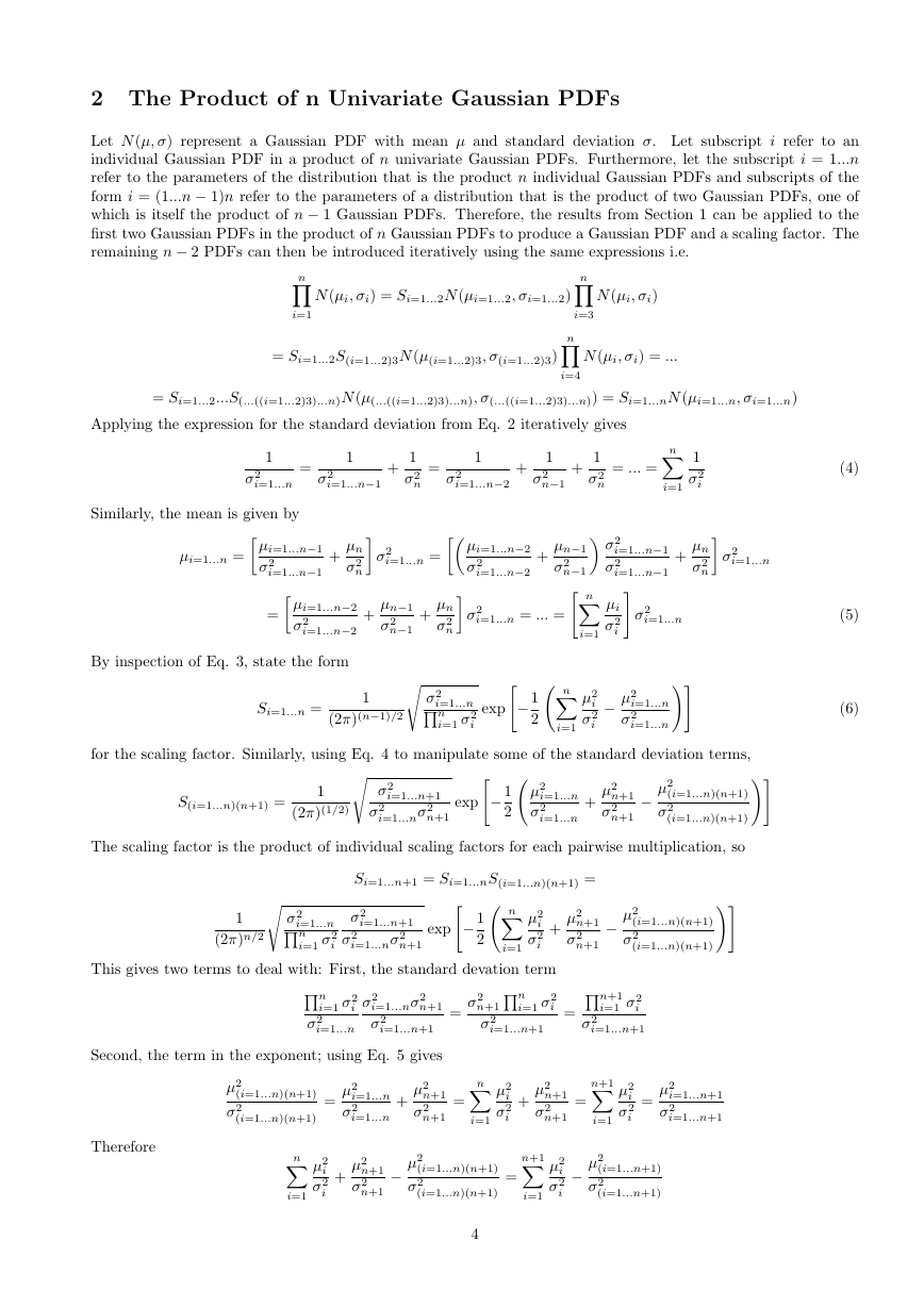
2 The Product of n Univariate Gaussian PDFs Let N (µ, σ) represent a Gaussian PDF with mean µ and standard deviation σ. Let subscript i refer to an individual Gaussian PDF in a product of n univariate Gaussian PDFs. Furthermore, let the subscript i = 1...n refer to the parameters of the distribution that is the product n individual Gaussian PDFs and subscripts of the form i = (1...n − 1)n refer to the parameters of a distribution that is the product of two Gaussian PDFs, one of which is itself the product of n − 1 Gaussian PDFs. Therefore, the results from Section 1 can be applied to the ﬁrst two Gaussian PDFs in the product of n Gaussian PDFs to produce a Gaussian PDF and a scaling factor. The remaining n − 2 PDFs can then be introduced iteratively using the same expressions i.e. N (µi, σi) = Si=1...2N (µi=1...2, σi=1...2) N (µi, σi) n Yi=1 = Si=1...2S(i=1...2)3N (µ(i=1...2)3, σ(i=1...2)3) N (µi, σi) = ... n Yi=3 Yi=4 n = Si=1...2...S(...((i=1...2)3)...n)N (µ(...((i=1...2)3)...n), σ(...((i=1...2)3)...n)) = Si=1...nN (µi=1...n, σi=1...n) (4) (5) (6) Applying the expression for the standard deviation from Eq. 2 iteratively gives 1 σ2 i=1...n = 1 σ2 i=1...n−1 + 1 σ2 n = 1 σ2 i=1...n−2 + 1 σ2 n−1 + 1 σ2 n = ... = n Xi=1 1 σ2 i Similarly, the mean is given by µi=1...n = µi=1...n−1 i=1...n−1 σ2 + µn σ2 n σ2 i=1...n = µi=1...n−2 i=1...n−2 σ2 i=1...n−1 i=1...n−1 + µn σ2 n σ2 i=1...n + σ2 µn−1 σ2 n−1 σ2 i=1...n = ... =" n Xi=1 µi σ2 i # σ2 i=1...n = µi=1...n−2 i=1...n−2 σ2 + µn−1 σ2 n−1 + By inspection of Eq. 3, state the form µn σ2 n σ2 Si=1...n = 1 (2π)(n−1)/2s σ2 Qn i=1...n i=1 σ2 i exp"− 1 2 n Xi=1 µ2 i i − σ2 µ2 σ2 i=1...n i=1...n!# for the scaling factor. Similarly, using Eq. 4 to manipulate some of the standard deviation terms, S(i=1...n)(n+1) = 1 (2π)(1/2)s σ2 i=1...n+1 σ2 i=1...nσ2 n+1 exp"− 1 2 µ2 σ2 i=1...n i=1...n + n+1 µ2 n+1 − σ2 µ2 σ2 (i=1...n)(n+1) (i=1...n)(n+1)!# The scaling factor is the product of individual scaling factors for each pairwise multiplication, so Si=1...n+1 = Si=1...nS(i=1...n)(n+1) = This gives two terms to deal with: First, the standard devation term σ2 i=1...n+1 i=1...nσ2 σ2 n+1 exp"− 1 2 n Xi=1 µ2 i σ2 i + n+1 µ2 n+1 − σ2 µ2 σ2 (i=1...n)(n+1) (i=1...n)(n+1)!# i=1...n i=1 σ2 i 1 (2π)n/2s σ2 Qn Qn σ2 i=1 σ2 i i=1...n i=1...nσ2 σ2 σ2 i=1...n+1 n+1 = i=1 σ2 i σ2 n+1Qn σ2 i=1...n+1 = Qn+1 i=1 σ2 i i=1...n+1 σ2 Second, the term in the exponent; using Eq. 5 gives µ2 σ2 (i=1...n)(n+1) (i=1...n)(n+1) = µ2 σ2 i=1...n i=1...n + µ2 σ2 n+1 n+1 = µ2 i σ2 i n Xi=1 + µ2 σ2 n+1 n+1 = µ2 i σ2 i n+1 Xi=1 = µ2 σ2 i=1...n+1 i=1...n+1 Therefore µ2 i σ2 i n Xi=1 + n+1 µ2 n+1 − σ2 µ2 σ2 (i=1...n)(n+1) (i=1...n)(n+1) = n+1 Xi=1 µ2 i i − σ2 µ2 σ2 (i=1...n+1) (i=1...n+1) 4

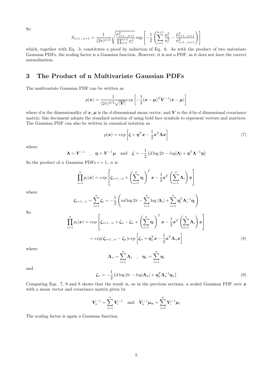
So Si=1...n+1 = 1 (2π)n/2s σ2 i=1...n+1 i=1 σ2 i Qn+1 exp"− 1 2 n+1 Xi=1 µ2 i i − σ2 µ2 σ2 i=1...n+1 i=1...n+1!# which, together with Eq. 3, constitutes a proof by induction of Eq. 6. As with the product of two univariate Gaussian PDFs, the scaling factor is a Gaussian function. However, it is not a PDF, as it does not have the correct normalisation. 3 The Product of n Multivariate Gaussian PDFs The multivariate Gaussian PDF can be written as p(x) = 1 (2π)d/2p|V | exp− 1 2 (x − µ)T V −1(x − µ) where d is the dimensionality of x, µ is the d-dimensional mean vector, and V is the d-by-d dimensional covariance matrix; this document adopts the standard notation of using bold face symbols to represent vectors and matrices. The Gaussian PDF can also be written in canonical notation as where Λ = V −1 , η = V −1µ and ζ = − So the product of n Gaussian PDFs i = 1...n is p(x) = expζ + ηT x − 1 2 xT Λx 1 2d log 2π − log|Λ| + ηT Λ−1η ηi!T x − xT n Xi=1 1 2 n n n 1 Yi=1 ζi=1...n = ζi = − pi(x) = exp ζi=1...n + n Xi=1 2 nd log 2π − Xi=1 Xi=1 pi(x) = exp ηi!T ζi=1...n + ζn − ζn + n Xi=1 = exp(ζi=1...n − ζn)expζn + ηT n x − Λ−1 Λi! x  i ηi! Λi! x  n ηT i Xi=1 xT n Xi=1 x − xT Λnx 1 2 1 2 log |Λi| + where So where and n Yi=1 (7) (8) (9) ηi n n Λn = Λi , ηn = Xi=1 Xi=1 2d log 2π − log|Λn| + ηT 1 n Λ−1 n ηn ζn = − Comparing Eqs. 7, 9 and 8 shows that the result is, as in the previous sections, a scaled Gaussian PDF over x with a mean vector and covariance matrix given by V −1 n = n Xi=1 V −1 i and V −1 n µn = V −1 i µi n Xi=1 The scaling factor is again a Gaussian function. 5

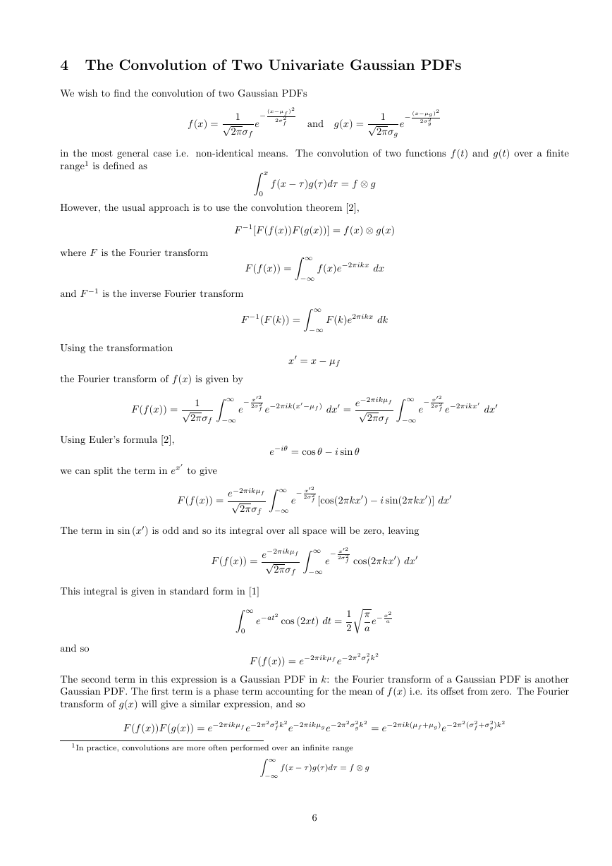
4 The Convolution of Two Univariate Gaussian PDFs We wish to ﬁnd the convolution of two Gaussian PDFs f (x) = 1 √2πσf − e (x−µf )2 2σ2 f and g(x) = (x−µg )2 2σ2 g 1 √2πσg − e in the most general case i.e. non-identical means. The convolution of two functions f (t) and g(t) over a ﬁnite range1 is deﬁned as Z x 0 f (x − τ )g(τ )dτ = f ⊗ g However, the usual approach is to use the convolution theorem [2], where F is the Fourier transform F −1[F (f (x))F (g(x))] = f (x) ⊗ g(x) F (f (x)) =Z ∞ f (x)e−2πikx dx −∞ and F −1 is the inverse Fourier transform Using the transformation F −1(F (k)) =Z ∞ −∞ F (k)e2πikx dk x′ = x − µf the Fourier transform of f (x) is given by F (f (x)) = Using Euler’s formula [2], 1 √2πσf Z ∞ −∞ − x′2 2σ2 f e−2πik(x′−µf ) dx′ = e e−2πikµf √2πσf Z ∞ −∞ − x′2 2σ2 f e−2πikx′ e dx′ we can split the term in ex′ to give F (f (x)) = e−iθ = cos θ − i sin θ e−2πikµf √2πσf Z ∞ −∞ − x′2 2σ2 f [cos(2πkx′) − i sin(2πkx′)] dx′ e The term in sin (x′) is odd and so its integral over all space will be zero, leaving F (f (x)) = This integral is given in standard form in [1] e−2πikµf √2πσf Z ∞ −∞ − x′2 2σ2 f cos(2πkx′) dx′ e e−at2 cos (2xt) dt = Z ∞ 0 1 2r π a e− x2 a and so F (f (x)) = e−2πikµf e−2π2σ2 f k2 The second term in this expression is a Gaussian PDF in k: the Fourier transform of a Gaussian PDF is another Gaussian PDF. The ﬁrst term is a phase term accounting for the mean of f (x) i.e. its oﬀset from zero. The Fourier transform of g(x) will give a similar expression, and so F (f (x))F (g(x)) = e−2πikµf e−2π2σ2 f k2 e−2πikµg e−2π2σ2 gk2 1In practice, convolutions are more often performed over an inﬁnite range Z ∞ −∞ f (x − τ )g(τ )dτ = f ⊗ g 6 = e−2πik(µf +µg)e−2π2(σ2 f +σ2 g)k2

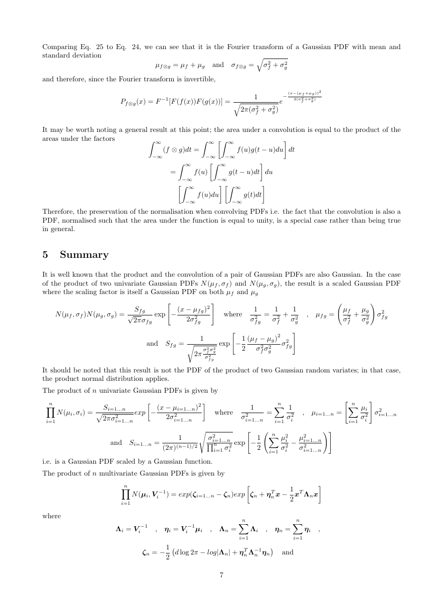
Comparing Eq. 25 to Eq. 24, we can see that it is the Fourier transform of a Gaussian PDF with mean and standard deviation and therefore, since the Fourier transform is invertible, µf ⊗g = µf + µg and σf ⊗g =qσ2 f + σ2 g Pf ⊗g(x) = F −1[F (f (x))F (g(x))] = (x−(µf +µg ))2 2(σ2 f +σ2 g ) − e 1 f + σ2 g) q2π(σ2 It may be worth noting a general result at this point; the area under a convolution is equal to the product of the areas under the factors Z ∞ −∞ −∞ −∞Z ∞ (f ⊗ g)dt =Z ∞ =Z ∞ f (u)Z ∞ f (u)duZ ∞ Z ∞ f (u)g(t − u)du dt g(t − u)dt du g(t)dt −∞ −∞ −∞ −∞ Therefore, the preservation of the normalisation when convolving PDFs i.e. the fact that the convolution is also a PDF, normalised such that the area under the function is equal to unity, is a special case rather than being true in general. 5 Summary It is well known that the product and the convolution of a pair of Gaussian PDFs are also Gaussian. In the case of the product of two univariate Gaussian PDFs N (µf , σf ) and N (µg, σg), the result is a scaled Gaussian PDF where the scaling factor is itself a Gaussian PDF on both µf and µg N (µf , σf )N (µg, σg) = Sf g√2πσf g exp"− (x − µf g)2 2σ2 f g # where exp"− g 1 2 1 σ2 f g = 1 σ2 f + 1 σ2 g , µf g = µf σ2 f + (µf − µg)2 σ2 f σ2 g σ2 f g# µg σ2 g! σ2 f g and Sf g = 1 r2π σ2 f σ2 σ2 f g It should be noted that this result is not the PDF of the product of two Gaussian random variates; in that case, the product normal distribution applies. The product of n univariate Gaussian PDFs is given by N (µi, σi) = n Yi=1 Si=1...n i=1...n p2πσ2 exp− and Si=1...n = (x − µi=1...n)2 2σ2 i=1...n where 1 σ2 i=1...n 1 (2π)(n−1)/2s σ2 Qn i=1...n i=1 σ2 i exp"− n = Xi=1 2 n Xi=1 1 1 σ2 i µ2 i i − σ2 µi σ2 i # σ2 i=1...n , µi=1...n =" n Xi=1 i=1...n!# i=1...n µ2 σ2 i.e. is a Gaussian PDF scaled by a Gaussian function. The product of n multivariate Gaussian PDFs is given by n Yi=1 N (µi, V −1 i ) = exp(ζi=1...n − ζn)expζn + ηT n x − 1 2 xT Λnx where Λi = V −1 i , ηi = V −1 i µi , Λn = Xi=1 2d log 2π − log|Λn| + ηT 1 n ζn = − 7 n Λi , ηn = ηi , n Xi=1 and Λ−1 n ηn

ζi=1...n = ζi = − 1 2 nd log 2π − n Xi=1 n Xi=1 log |ηi| + ηT i Λ−1 i ηi! n Xi=1 i.e. a Gaussian PDF scaled by a Gaussian function. The convolution of two Gaussian PDFs is a Gaussian PDF with mean and standard deviation µf ⊗g = µf + µg and σf ⊗g =qσ2 f + σ2 g These results can be useful in a number of applications; for example, the convolution of Gaussian distributions freqently occurs in smoothing applied as an intermadiate step in various machine vision algorithms. Products of Gaussian PDFs may occur during the application of Bayes theorem, and in some problems related to Gaussian processes. 6 Acknoweldgements Thanks are due to David Kirchheimer, University of Bristol, for pointing out the importance of the product of an arbitrary number of Gaussian PDFs and providing Matlab code for numerical testing of the results. Thanks are also due to Thomas Dent, Institute for Gravitational Physics (Albert Einstein Institute), Hannover, Germany, for pointing out several typographical errors. References [1] M Abramowitz and I A Stegun. Handbook of Mathematical Functions. National Bureau of Standards, Wash- ington DC, 1972. [2] M L Boas. Mathematical Methods in the Physical Sciences. John Wiley and Sons Ltd., 1983. 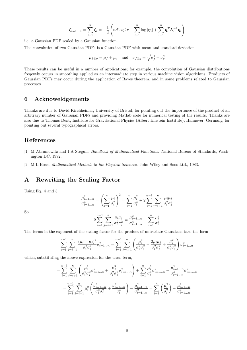A Rewriting the Scaling Factor Using Eq. 4 and 5 So µ2 σ4 i=1...n i=1...n = n Xi=1 i !2 µi σ2 = µ2 i σ4 i n Xi=1 + 2 n−1 Xi=1 n Xj=i+1 µiµj σ2 i σ2 j 2 n−1 Xi=1 n Xj=i+1 µiµj i σ2 σ2 j = i=1...n µ2 i=1...n − σ4 µ2 i σ4 i n Xi=1 The terms in the exponent of the scaling factor for the product of univariate Gaussians take the form n−1 Xi=1 n Xj=i+1 (µi − µj)2 σ2 i σ2 j σ2 i=1...n = n−1 Xi=1 n Xj=i+1 µ2 i σ2 i σ2 j − 2µiµj σ2 i σ2 j + µ2 j σ2 i σ2 j! σ2 i=1...n which, substituting the above expression for the cross term, = n−1 Xi=1 = n i σ2 i σ2 j Xj=i+1 µ2 Xj=i+1 Xi=1 n−1 µ2 n σ2 i=1...n! + i ! − µ2 σ2 σ2 i=1...n σ4 µ2 i σ4 i n Xi=1 σ2 i=1...n − µ2 σ4 i=1...n i=1...n σ2 i=1...n i=1...n i=1...n = n Xi=1 µ2 i σ2 i − µ2 σ2 i=1...n i=1...n σ2 i=1...n + µ2 j σ2 i σ2 j i σ2 i=1...n σ2 i σ2 j + 8

分享到：

赞收藏

资料库

正态分布乘积等于正态分布的证明.pdf

相关推荐

课程资源

热门标签

最新资料