metabolomics_data_using_OPLS-DA.pdf-资料库

f706e147-48a1-41e5-bf54-2fbed5bbccb6.pdf-第1页.png

第1页 / 共8页

f706e147-48a1-41e5-bf54-2fbed5bbccb6.pdf-第2页.png

第2页 / 共8页

f706e147-48a1-41e5-bf54-2fbed5bbccb6.pdf-第3页.png

第3页 / 共8页

f706e147-48a1-41e5-bf54-2fbed5bbccb6.pdf-第4页.png

第4页 / 共8页

f706e147-48a1-41e5-bf54-2fbed5bbccb6.pdf-第5页.png

第5页 / 共8页

f706e147-48a1-41e5-bf54-2fbed5bbccb6.pdf-第6页.png

第6页 / 共8页

f706e147-48a1-41e5-bf54-2fbed5bbccb6.pdf-第7页.png

第7页 / 共8页

f706e147-48a1-41e5-bf54-2fbed5bbccb6.pdf-第8页.png

第8页 / 共8页

Analysing NMR Metabolomics data using OPLS-DA Background A gene encoding MYB transcription factor, with unknown function, PttMYB76, was selected from a library of poplar trees for metabolomic characterization of the growth process in Poplar trees. Objective The objective of this exercise is to shed some light on how PCA and OPLS-DA may be used in state-of- the-art Metabolomics. In particular, the objectives are to: • Demonstrate how to analyze metabolomics data from two sets of samples representing one control group and one treated group o Using PCA to review data, identify patterns and trends • Demonstrate how to identify differences and putative biomarkers in different sample groups and compare the strength of OPLS-DA compared to PCA o Using OPLS-DA • Describe the model diagnostics of an OPLS-DA model Data In total, the data set contains N = 57 observations, 6 trees divided into segments of 8 by the internode of the tree plus analytical replicates and K = 655 variables (1H-NMR chemical shift regions bucket with 0.02ppm). The internode represents the growth direction of a plant. Internode 1 is the top of the plant and 8 is the bottom. The observations (trees) are divided in two groups (“classes”): • MYB76 poplar plant (Ai, Bi, Ci)- Class 2 • Wild type Poplar plant (Di, Ei, Fi)- Class 1 The name settings A, B, C corresponds to MYB76 plants and D, E, F to the wild type (control) plants. The i after the letter corresponds to the internode number of the plant. The last 12 experiments in the dataset are analytical replicates i.e. samples that were run twice in the spectrometer. The analytical replicates are marked with r1 or r2 after the internode number. The plant material was analyzed by a 500 MHz NMR spectrometer equipped with a HR/MAS probe. The 1H NMR spectra were reduced by binning all of the data points over a 0.02 ppm region. Data points between 4.2- 5.6 ppm, corresponding to water resonances, were excluded, leaving a total of 655 NMR spectral regions as variables for the multivariate modelling. A more detailed description of the experimental conditions is found in [1]. 1 S. Wiklund et.al A new metabonomic strategy for analysing the growth process of the poplar tree. Plant Biotechnology Journal 2005 3 pp 353-362 SIMCA Tutorial Analysing NMR Metabolomics data using OPLS-DA •••• 1

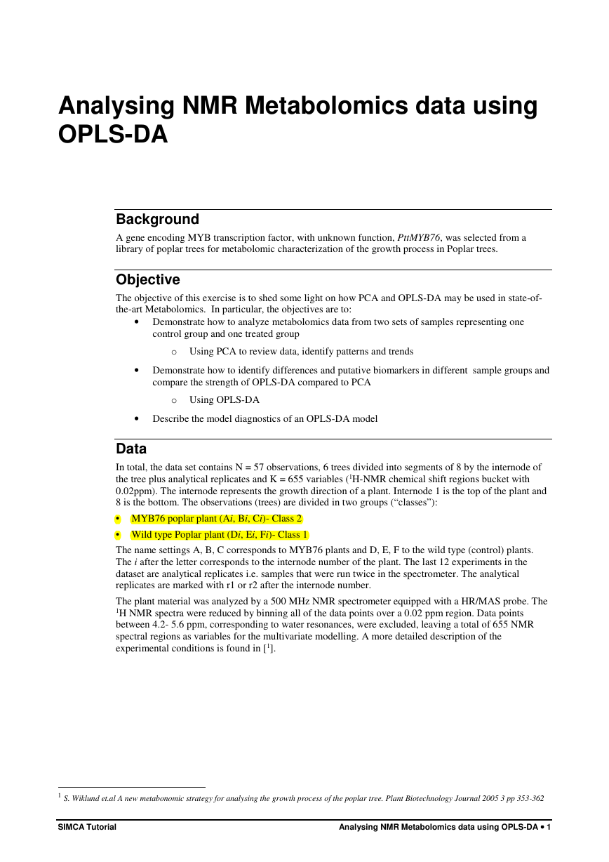
Import data Create a SIMCA project using file NMR METABOLOMICS.xls. The imported file must be transposed. Use Edit: Transpose as demonstrated in the figure: Mark the first row and select primary variable id. Make sure that the first column is marked as primary observation IDs. In the second column you can see that the data has been extended to designate the different classes, Set this as secondary ID. This secondary ID will be used to define classes in SIMCA. 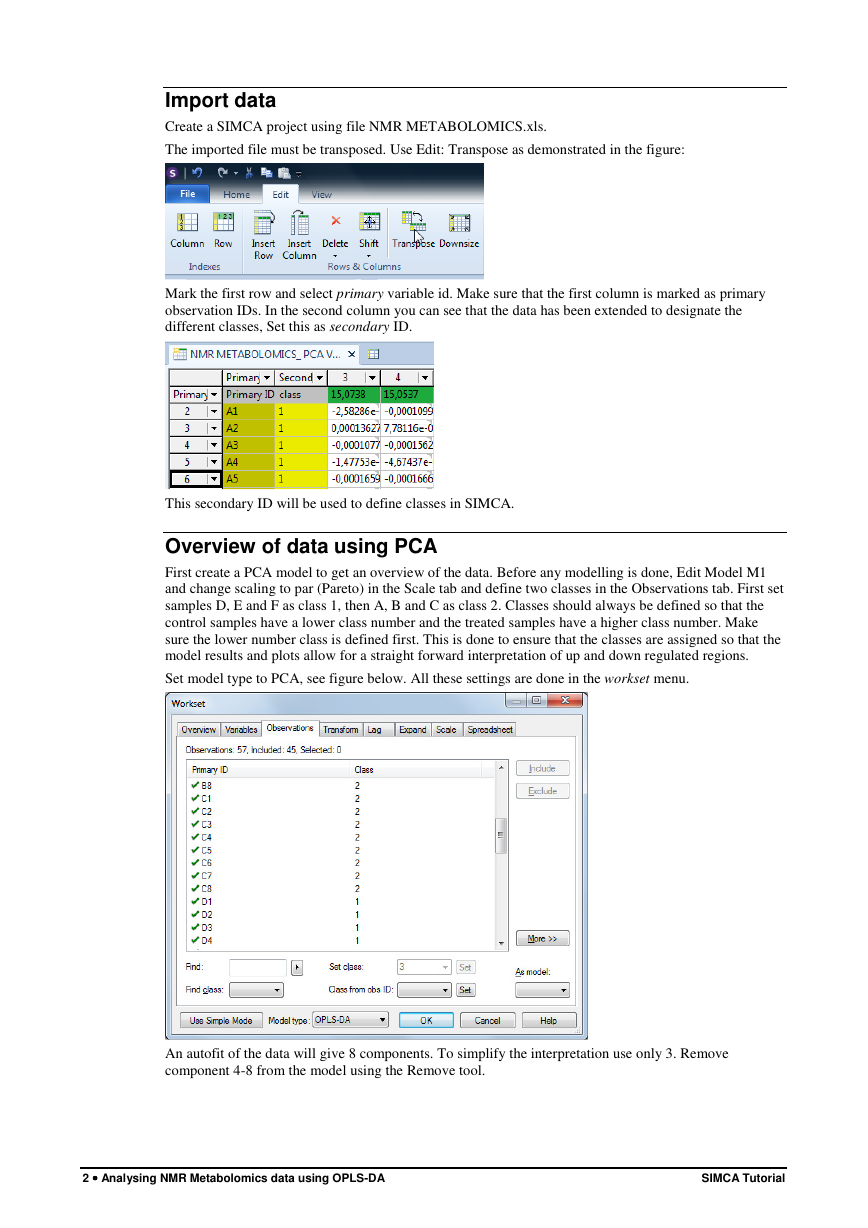Overview of data using PCA First create a PCA model to get an overview of the data. Before any modelling is done, Edit Model M1 and change scaling to par (Pareto) in the Scale tab and define two classes in the Observations tab. First set samples D, E and F as class 1, then A, B and C as class 2. Classes should always be defined so that the control samples have a lower class number and the treated samples have a higher class number. Make sure the lower number class is defined first. This is done to ensure that the classes are assigned so that the model results and plots allow for a straight forward interpretation of up and down regulated regions. Set model type to PCA, see figure below. All these settings are done in the workset menu. An autofit of the data will give 8 components. To simplify the interpretation use only 3. Remove component 4-8 from the model using the Remove tool. 2 •••• Analysing NMR Metabolomics data using OPLS-DA SIMCA Tutorial

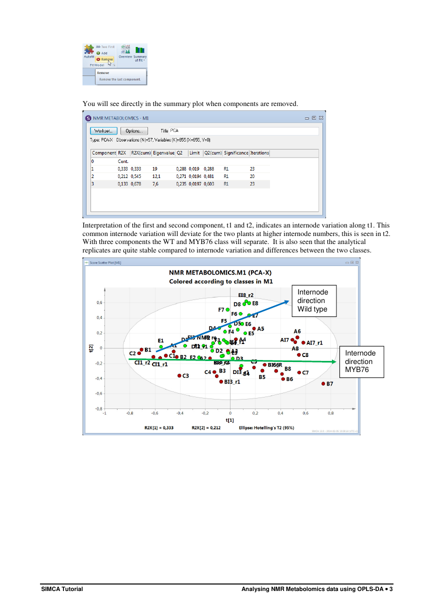
You will see directly in the summary plot when components are removed. Interpretation of the first and second component, t1 and t2, indicates an internode variation along t1. This common internode variation will deviate for the two plants at higher internode numbers, this is seen in t2. With three components the WT and MYB76 class will separate. It is also seen that the analytical replicates are quite stable compared to internode variation and differences between the two classes. Internode direction Wild type Internode direction MYB76 SIMCA Tutorial Analysing NMR Metabolomics data using OPLS-DA •••• 3

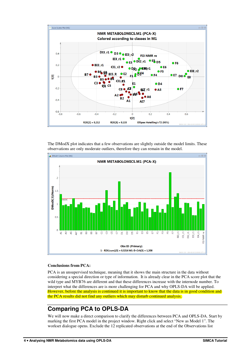
The DModX plot indicates that a few observations are slightly outside the model limits. These observations are only moderate outliers, therefore they can remain in the model. Conclusions from PCA: PCA is an unsupervised technique, meaning that it shows the main structure in the data without considering a special direction or type of information. It is already clear in the PCA score plot that the wild type and MYB76 are different and that these differences increase with the internode number. To interpret what the differences are is more challenging for PCA and why OPLS-DA will be applied. However, before the analysis is continued it is important to know that the data is in good condition and the PCA results did not find any outliers which may disturb continued analysis. Comparing PCA to OPLS-DA We will now make a direct comparison to clarify the differences between PCA and OPLS-DA. Start by marking the first PCA model in the project window. Right click and select “New as Model 1”. The workset dialogue opens. Exclude the 12 replicated observations at the end of the Observations list 4 •••• Analysing NMR Metabolomics data using OPLS-DA SIMCA Tutorial

denoted r1 and r2. Model type should be PCA-X, press OK. Autofit the data and a 7 component model appears. The next step is to create an OPLS-DA model. Right click on model 2 and select “New as Model 2”. Change the model type to OPLS-DA at the bottom of the Workset window. Press OK. Autofit the model. A 1+4 OPLS model is created Plot scores and compare the results from the PCA model to the OPLS-DA model. What can be seen in the first OPLS-DA component? What can be seen in the orthogonal components? A basic requirement for all prediction modeling is that the model is reasonably good with a high Q2. Before doing any interpretation we need to check that the OPLS-DA model fulfils this requirement. In this example we got a Q2 of 0,941 which is very high, so we can proceed to do model interpretation. 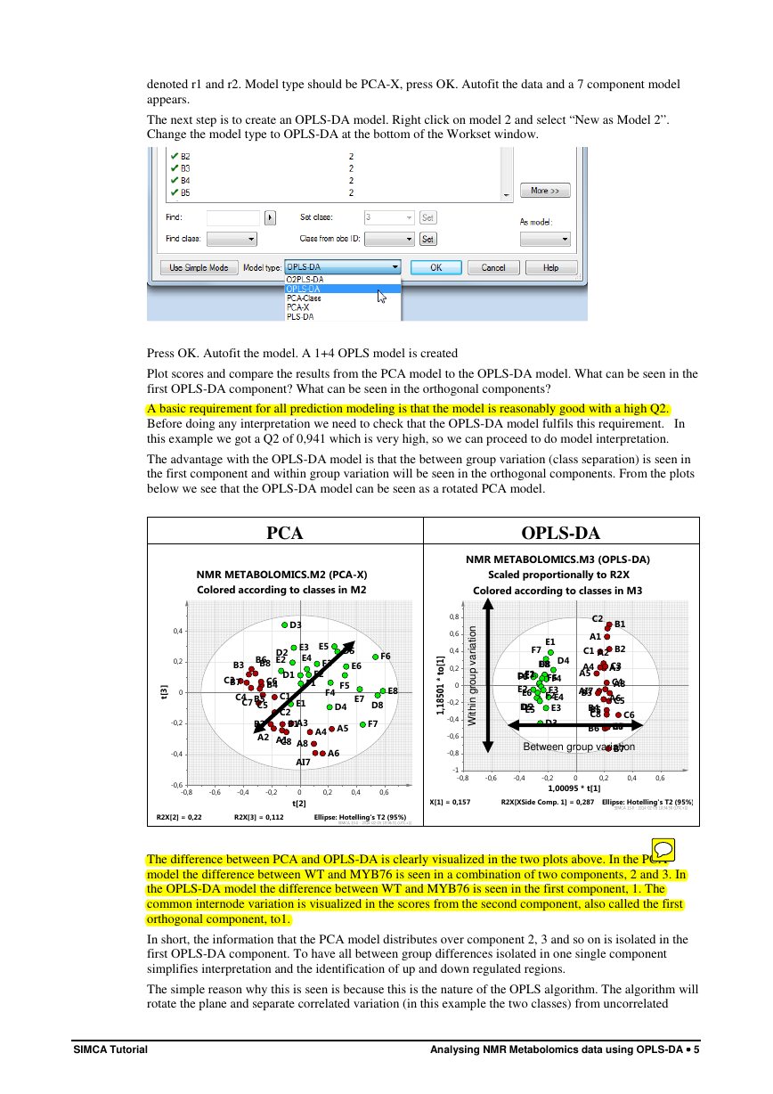The advantage with the OPLS-DA model is that the between group variation (class separation) is seen in the first component and within group variation will be seen in the orthogonal components. From the plots below we see that the OPLS-DA model can be seen as a rotated PCA model. PCA OPLS-DA NMR METABOLOMICS.M2 (PCA-X) Colored according to classes in M2 NMR METABOLOMICS.M3 (OPLS-DA) Scaled proportionally to R2X Colored according to classes in M3 D3 B3 B6 B8 D2 E2 E3 E4 E5 F3 C3 B7 D1 C6 B4 F2 F1 C4 C7 B5 C5 B2 A2 C1 C2 E1 B1 A3 A1 C8 A8 D5 E6 F5 F4 D4 E7 A4 A5 A6 AI7 n o i t a i r a v p u o r g n h i t i W F6 E8 D8 F7 0,8 0,6 0,4 0,2 0 -0,2 -0,4 -0,6 -0,8 -1 E1 F7 D4 D8 E8 F1 E7 D1 F6 E2 E6 D2 D5 E5 F4F5 F3 F2 E4 E3 D3 C2 A1 C1 A2 A4 A5 AI7 B3 B4B5 C8 B6 B1 B2 C3 A3 C4 A8 A6 C5 C6 B8 C7 Between group variation B7 -0,8 -0,6 -0,4 -0,2 0 0,2 0,4 0,6 1,00095 * t[1] 0,4 0,2 ] 3 [ t 0 -0,2 -0,4 -0,6 -0,8 -0,6 -0,4 -0,2 0 0,2 0,4 0,6 R2X[2] = 0,22 R2X[3] = 0,112 Ellipse: Hotelling's T2 (95%) t[2] R2X[1] = 0,157 R2X[XSide Comp. 1] = 0,287 Ellipse: Hotelling's T2 (95%) The difference between PCA and OPLS-DA is clearly visualized in the two plots above. In the PCA model the difference between WT and MYB76 is seen in a combination of two components, 2 and 3. In the OPLS-DA model the difference between WT and MYB76 is seen in the first component, 1. The common internode variation is visualized in the scores from the second component, also called the first orthogonal component, to1. In short, the information that the PCA model distributes over component 2, 3 and so on is isolated in the first OPLS-DA component. To have all between group differences isolated in one single component simplifies interpretation and the identification of up and down regulated regions. The simple reason why this is seen is because this is the nature of the OPLS algorithm. The algorithm will rotate the plane and separate correlated variation (in this example the two classes) from uncorrelated SIMCA Tutorial Analysing NMR Metabolomics data using OPLS-DA •••• 5

variation between X and Y. Uncorrelated variation is also called orthogonal variation and is not related to the observed response Y. Technical Note: As OPLS rotates the first score vector t1 when additional components are computed the t1 vs. to1 plot changes when you add additional components to the model. Make sure that the model is optimized by using cross validation. Do NOT optimize the model by visualizing the class separation from the score plot. 6 •••• Analysing NMR Metabolomics data using OPLS-DA SIMCA Tutorial

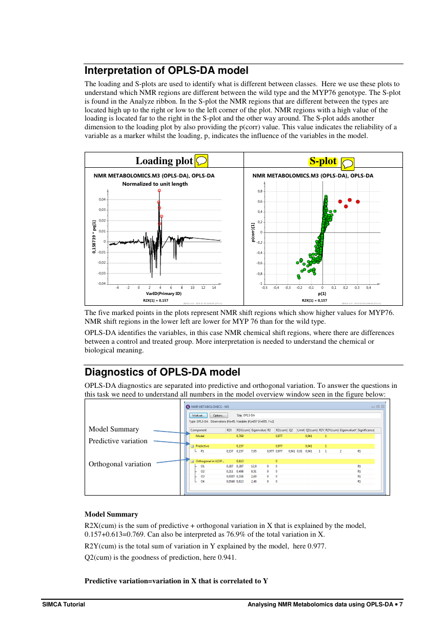
Interpretation of OPLS-DA model The loading and S-plots are used to identify what is different between classes. Here we use these plots to understand which NMR regions are different between the wild type and the MYP76 genotype. The S-plot is found in the Analyze ribbon. In the S-plot the NMR regions that are different between the types are located high up to the right or low to the left corner of the plot. NMR regions with a high value of the loading is located far to the right in the S-plot and the other way around. The S-plot adds another dimension to the loading plot by also providing the p(corr) value. This value indicates the reliability of a variable as a marker whilst the loading, p, indicates the influence of the variables in the model. Loading plot S-plot NMR METABOLOMICS.M3 (OPLS-DA), OPLS-DA NMR METABOLOMICS.M3 (OPLS-DA), OPLS-DA Normalized to unit length ] 1 [ q p * 9 3 7 8 5 1 0 , 0,04 0,03 0,02 0,01 0 -0,01 -0,02 -0,03 -0,04 ] 1 [ ) r r o c ( p 0,8 0,6 0,4 0,2 0 -0,2 -0,4 -0,6 -0,8 -1 -4 -2 0 2 4 6 8 10 12 14 -0,5 -0,4 -0,3 -0,2 -0,1 0 0,1 0,2 0,3 0,4 VarID(Primary ID) R2X[1] = 0,157 p[1] R2X[1] = 0,157 The five marked points in the plots represent NMR shift regions which show higher values for MYP76. NMR shift regions in the lower left are lower for MYP 76 than for the wild type. OPLS-DA identifies the variables, in this case NMR chemical shift regions, where there are differences between a control and treated group. More interpretation is needed to understand the chemical or biological meaning. 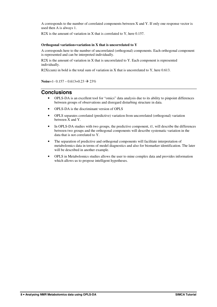Diagnostics of OPLS-DA model OPLS-DA diagnostics are separated into predictive and orthogonal variation. To answer the questions in this task we need to understand all numbers in the model overview window seen in the figure below: Model Summary Predictive variation Orthogonal variation Model Summary R2X(cum) is the sum of predictive + orthogonal variation in X that is explained by the model, 0.157+0.613=0.769. Can also be interpreted as 76.9% of the total variation in X. R2Y(cum) is the total sum of variation in Y explained by the model, here 0.977. Q2(cum) is the goodness of prediction, here 0.941. Predictive variation=variation in X that is correlated to Y SIMCA Tutorial Analysing NMR Metabolomics data using OPLS-DA •••• 7

A corresponds to the number of correlated components between X and Y. If only one response vector is used then A is always 1. R2X is the amount of variation in X that is correlated to Y, here 0.157. Orthogonal variation=variation in X that is uncorrelated to Y A corresponds here to the number of uncorrelated (orthogonal) components. Each orthogonal component is represented and can be interpreted individually. R2X is the amount of variation in X that is uncorrelated to Y. Each component is represented individually. R2X(cum) in bold is the total sum of variation in X that is uncorrelated to Y, here 0.613. Noise=1- 0.157 – 0.613=0.23 23% Conclusions • OPLS-DA is an excellent tool for “omics” data analysis due to its ability to pinpoint differences between groups of observations and disregard disturbing structure in data. • OPLS-DA is the discriminant version of OPLS • OPLS separates correlated (predictive) variation from uncorrelated (orthogonal) variation between X and Y. • In OPLS-DA studies with two groups, the predictive component, t1, will describe the differences between two groups and the orthogonal components will describe systematic variation in the data that is not correlated to Y. • The separation of predictive and orthogonal components will facilitate interpretation of metabolomics data in terms of model diagnostics and also for biomarker identification. The later will be described in another example. • OPLS in Metabolomics studies allows the user to mine complex data and provides information which allows us to propose intelligent hypotheses. 8 •••• Analysing NMR Metabolomics data using OPLS-DA SIMCA Tutorial

资料库

metabolomics_data_using_OPLS-DA.pdf

相关推荐

课程资源

热门标签

最新资料