Published for SISSA by
Springer
Received: February 13, 2016
Accepted: March 27, 2016
Published: April 1, 2016
The spectrum in the Sachdev-Ye-Kitaev model
Joseph Polchinski and Vladimir Rosenhaus
Kavli Institute for Theoretical Physics, University of California,
Santa Barbara, CA 93106, U.S.A.
E-mail: joep@kitp.ucsb.edu, vladr@kitp.ucsb.edu
Abstract: The SYK model consists of N 1 fermions in 0 + 1 dimensions with a
random, all-to-all quartic interaction. Recently, Kitaev has found that the SYK model is
maximally chaotic and has proposed it as a model of holography. We solve the Schwinger-
Dyson equation and compute the spectrum of two-particle states in SYK, nding both
a continuous and discrete tower. The four-point function is expressed as a sum over the
spectrum. The sum over the discrete tower is evaluated.
Keywords: 1/N Expansion, AdS-CFT Correspondence, Field Theories in Lower Dimen-
sions, M(atrix) Theories
ArXiv ePrint: 1601.06768
Open Access, c The Authors.
Article funded by SCOAP3.
doi:10.1007/JHEP04(2016)001
JHEP04(2016)001�
Contents
1 Introduction
2 Two-point function
3 Spectrum
3.1 Eigenvalues
3.2 SL(2;R) and all eigenvectors
3.3 Directly nding the eigenvectors
3.4 A complete set of eigenvectors
4 Four-point function
A Integrals in eigenvalue computation
B Eigenvectors and boundary terms
C Integral in eigenvector computation
D Integrals of products of Bessel functions
1
2
5
6
7
8
9
11
17
18
19
20
Introduction
1
The Sachdev-Ye-Kitaev model (SYK) [1, 2] is a 0 + 1 dimensional model of N 1 fermions
with an all-to-all random quartic interaction. SYK has three notable features:
Solvable at strong coupling. At large N one can sum all Feynman diagrams, and
thereby compute correlation functions at strong coupling.
Maximally chaotic. Chaos is quantied by the Lyapunov exponent, which is dened by
an out-of-time-order four-point function [3, 4]. The Lyapunov exponent of a black
hole in Einstein gravity is 2= [4{6], where is the inverse temperature. This is
the maximal allowed Lyapunov exponent [7], and SYK saturates the bound [1].
Emergent conformal symmetry. In the context of the two-point function, there is
emergent conformal symmetry at low energies [1, 8{10].
Due the scarcity of nontrivial systems which can be solved at strong coupling, the rst
item is already enough to make the model worthy of study. The combination of the rst
and the second items is remarkable and surprising. In the context of classical systems, solv-
ability usually means integrability, which is mutually exclusive from chaos. For a quantum
system, there is no such restriction, as SYK demonstrates. The third item implies that the
{ 1 {
JHEP04(2016)001�
model has some kind of holographic dual. The second item strongly suggests this dual is
Einstein gravity in some form. The combination of all three items would appear to poten-
tially place the model in the unique class of constituting a solvable model of holography.
SYK is a variant of the Sachdev-Ye model (SY) [2] that was introduced by Kitaev
in a series of seminars [1]. Kitaev made signicant advances in understanding the model,
connected the holographic study of chaos of Shenker and Stanford [5, 6, 11] to Lyapunov
exponents [3], and proposed SYK as a model of holography.
The main goal of this paper is to study the four-point function. This is also being
In section 2 we review the model, its two-point function, and
considered in [12, 13].
In section 3 we rst review the setup of the four-
the emergent conformal symmetry.
point function introduced in [1]. We then proceed to solve the Schwinger-Dyson equation
to compute the spectrum of two-particle states. We nd both a discrete tower and a
continuous tower.
In section 4 the four-point function is expressed as a sum over the
spectrum. The discrete part of the sum is explicitly evaluated. Some comments are made
on the breaking of conformal invariance.
2 Two-point function
The SYK model is given by the Hamiltonian [1],
NX
i;j;k;l=1
H =
1
4!
Jijkl ijkl ;
(2.1)
where j are Majorana fermions fi; jg = ij, and the model has quenched disorder with
the couplings Jijkl drawn from the distribution,
P (Jijkl) expN 3J 2
ijkl=12J 2 ;
leading to a disorder average of,
J 2
ijkl =
3!J 2
N 3 ;
Jijkl = 0 :
(2.2)
(2.3)
(2.4)
The expressions for the correlation functions that will follow will always be the result
after the disorder average has been performed. The Lagrangian trivially follows from the
Hamiltonian and is,
L = 1
2
j
d
dt
j H :
The couplings Jijkl have dimension 1, while the fermions i have dimension 0. The free
two-point function for the fermions is,
G0(t)ij hT i(t)j(0)i = 1
2
sgn(t)ij :
(2.5)
As a result of the disorder average, the anticommutation of the fermions, and large N , the
Feynman diagrams for the full (zero temperature) two-point function take a remarkably
{ 2 {
JHEP04(2016)001�
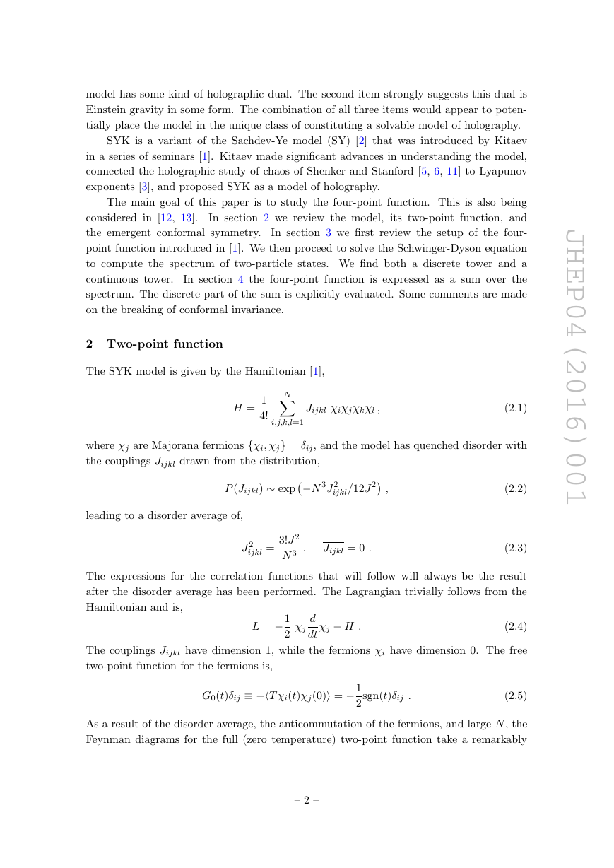
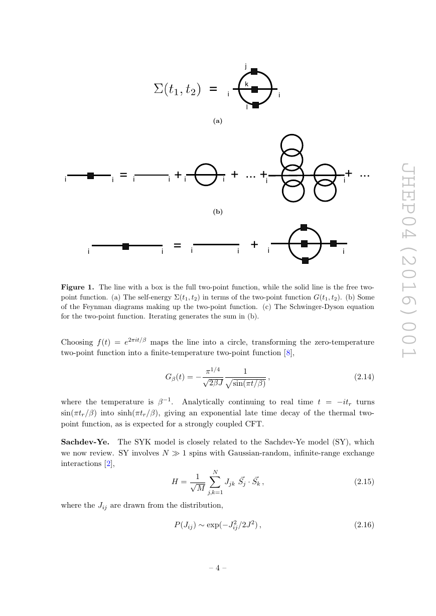
simple form. The self energy (t1; t2) (1PI) is expressed in terms of the two-point function
G(t1; t2) (see gure 1a)
(t1; t2) = J 2G(t1; t2)3 :
Expressing the two-point function as a sum of the 1PI diagrams,
G(i!)1 = i! (i!) :
(2.6)
(2.7)
The equations (2.6) and (2.7) fully determine the two-point function. Their solution is only
known in the limit of low energies. In this limit, one may drop the i! in (2.7), leading the
Fourier transform of (2.7) to become
(2.8)
(2.9)
(2.10)
Z
Z
dt G(t1; t)(t; t2) = (t1 t2) :
Combining (2.8) with (2.6) gives an integral equation for G(t1; t2),
J 2
dt G(t1; t)G(t; t2)3 = (t1 t2) ;
which one can check is solved by [2],
G(t) =
1
1=4
4J 2
1pjtj sgn(t) :
The solution (2.10) for the Euclidean two-point function is valid at low energies, or equiva-
lently, at strong coupling: the time separation t should satisfy Jjtj 1. On the basis of the
two-point function, it appears that the theory ows to an IR conformal xed point, with
the fermions acquiring an anomalous dimension = 1=4. The above equations (2.6), (2.7)
determining the two-point function can either be found from the Feynman diagrams, as
has been done here following ref. [1], or equivalently by performing the disorder average
via the replica trick and evaluating the saddle point of the action [2, 14].
An equivalent way to nd the two-point function is from the Schwinger-Dyson equation
in the form (see gure 1c),
G(t) = G0(t) + J 2
Z
dt1dt2 G0(t1)G(t1; t2)3G(t2; t) :
(2.11)
In the IR, one may drop the left-hand side, and nd the solution (2.10). The late time
decay of G(t), as compared to the constant behavior of G0(t), demonstrates that dropping
that left-hand side in (2.11) was self-consistent.
To go to nite temperature one uses the conformal invariance of the Schwinger-Dyson
equation (2.9) [1, 8]. Suppose G(1; 2) solves (2.9),
J 2
d G(1; )G(; 2)3 = (1 2) :
(2.12)
Z
Consider an arbitrary time reparameterization, = f (t). One can check that (2.12)
transforms into (2.9) provided one lets
G(t1; t2) = j@1f (t1)@2f (t2)j1=4G(1; 2) :
(2.13)
{ 3 {
JHEP04(2016)001�
(a)
(b)
Figure 1. The line with a box is the full two-point function, while the solid line is the free two-
point function. (a) The self-energy (t1; t2) in terms of the two-point function G(t1; t2). (b) Some
of the Feynman diagrams making up the two-point function. (c) The Schwinger-Dyson equation
for the two-point function. Iterating generates the sum in (b).
Choosing f (t) = e2it= maps the line into a circle, transforming the zero-temperature
two-point function into a nite-temperature two-point function [8],
G(t) = 1=4p
2J
1psin(t=)
;
(2.14)
where the temperature is 1. Analytically continuing to real time t = itr turns
sin(tr=) into sinh(tr=), giving an exponential late time decay of the thermal two-
point function, as is expected for a strongly coupled CFT.
Sachdev-Ye. The SYK model is closely related to the Sachdev-Ye model (SY), which
we now review. SY involves N 1 spins with Gaussian-random, innite-range exchange
interactions [2],
NX
j;k=1
H =
1p
M
Jjk ~Sj ~Sk ;
where the Jij are drawn from the distribution,
P (Jij) exp(J 2
ij=2J 2) ;
{ 4 {
(2.15)
(2.16)
JHEP04(2016)001=jklii+=+ ... ++ ...iiiiiiii+=iiiiii�
and the spins are in some representation of SU(M ). The choice of SU(2) was studied
by Bray and Moore [15], and it was numerically found to have spin-glass order at zero
temperature. Sachdev and Ye [2] considered (2.15) in an arbitrary representation of SU(M ),
obtaining analytic control over (2.15) in the limit M 1. The correlators in SY are
obtained by representing the spins in terms of fermions [2],
= cy
S
c;
cy
c = nb ;
(2.17)
X
where nb denotes the number of columns in the Young tableaux characterizing the repre-
sentation of SU(M ), and (2.17) holds at each site. Under the mapping (2.17) the Hamil-
tonian (2.15) is transformed into,
NX
MX
i;j=1
;=1
H =
1p
M
Jij c
y
ic
y
jc
i c
j ;
(2.18)
which, like the SYK Hamiltonian (2.1), is quartic in the fermions. Depending on the
representation of SU(M ), the ground state may or may not be a spin glass. One choice
of representation which was shown in [16] to avoid a spin glass phase is one with a Young
tableaux that has nb = O(1) columns and O(M ) rows, where M 1 [2]. In order to a
have a system that can serve as a model of holography, it is important that there not be
a spin-glass phase [4].1 For SYK, a spin glass phase is manifestly avoided, as the fermions
can not condense at a site (unlike the case of SY where the the fermions have an additional
gauge index ) [14]. SYK is simpler than SY, in that it only requires a single scaling limit
N ! 1, while SY also requires M ! 1. On the other hand, it may be useful to study SY
as well, as it has a 2-index coupling, which may t better with a bulk string theory than
the 4-index coupling Jijkl in SYK.
3 Spectrum
In this section we turn to the study of the four-point function,
hi(t1)i(t2)j(t3)j(t4)i :
(3.1)
The leading order connected piece scales as 1=N . As with the two-point function, the large
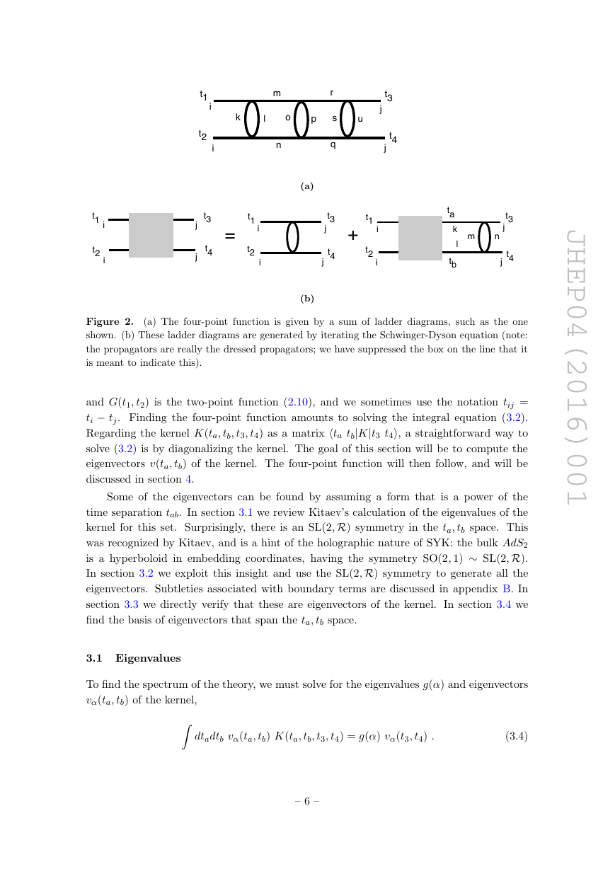
N structure of the four-point function is remarkably simple. At leading order, it is given
entirely by the ladder diagrams shown in gure 2 [1].
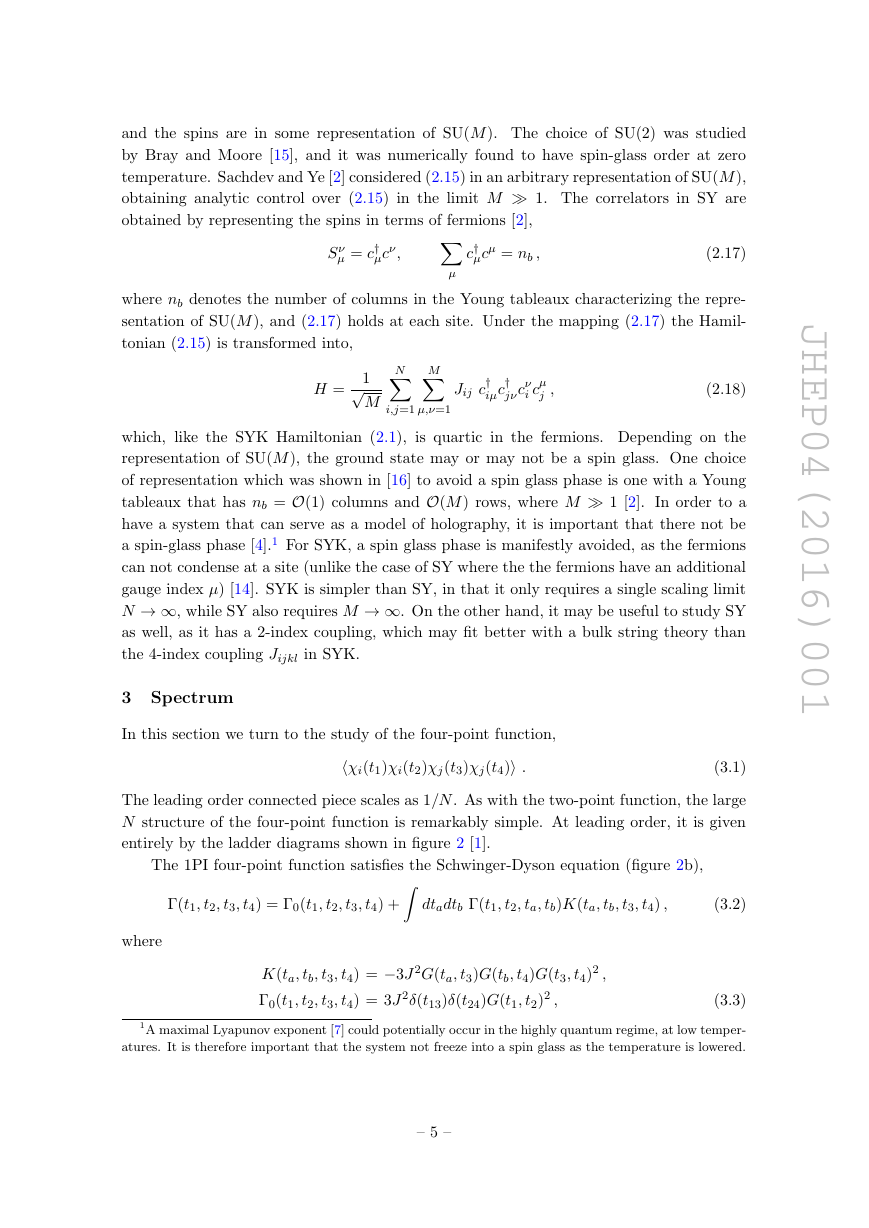
The 1PI four-point function satises the Schwinger-Dyson equation (gure 2b),
Z
(t1; t2; t3; t4) = 0(t1; t2; t3; t4) +
where
dtadtb (t1; t2; ta; tb)K(ta; tb; t3; t4) ;
(3.2)
K(ta; tb; t3; t4) = 3J 2G(ta; t3)G(tb; t4)G(t3; t4)2 ;
0(t1; t2; t3; t4) = 3J 2(t13)(t24)G(t1; t2)2 ;
(3.3)
1A maximal Lyapunov exponent [7] could potentially occur in the highly quantum regime, at low temper-
atures. It is therefore important that the system not freeze into a spin glass as the temperature is lowered.
{ 5 {
JHEP04(2016)001�
(a)
(b)
Figure 2.
(a) The four-point function is given by a sum of ladder diagrams, such as the one
shown. (b) These ladder diagrams are generated by iterating the Schwinger-Dyson equation (note:
the propagators are really the dressed propagators; we have suppressed the box on the line that it
is meant to indicate this).
and G(t1; t2) is the two-point function (2.10), and we sometimes use the notation tij =
ti tj. Finding the four-point function amounts to solving the integral equation (3.2).
Regarding the kernel K(ta; tb; t3; t4) as a matrix hta tbjKjt3 t4i, a straightforward way to
solve (3.2) is by diagonalizing the kernel. The goal of this section will be to compute the
eigenvectors v(ta; tb) of the kernel. The four-point function will then follow, and will be
discussed in section 4.
Some of the eigenvectors can be found by assuming a form that is a power of the
time separation tab. In section 3.1 we review Kitaev’s calculation of the eigenvalues of the
kernel for this set. Surprisingly, there is an SL(2;R) symmetry in the ta; tb space. This
was recognized by Kitaev, and is a hint of the holographic nature of SYK: the bulk AdS2
is a hyperboloid in embedding coordinates, having the symmetry SO(2; 1) SL(2;R).
In section 3.2 we exploit this insight and use the SL(2;R) symmetry to generate all the
eigenvectors. Subtleties associated with boundary terms are discussed in appendix B. In
section 3.3 we directly verify that these are eigenvectors of the kernel. In section 3.4 we
nd the basis of eigenvectors that span the ta; tb space.
3.1 Eigenvalues
To nd the spectrum of the theory, we must solve for the eigenvalues g() and eigenvectors
v(ta; tb) of the kernel,Z
dtadtb v(ta; tb) K(ta; tb; t3; t4) = g() v(t3; t4) :
(3.4)
{ 6 {
JHEP04(2016)001iijjt1t2t3t4klmnopqrsu+=iijjiijjiijjt1t2t3t4t1t2t3t4t1t2tat3t4tbklmn�
Schematically, we can write (3.4) as,
One set of eigenvectors that satisfy (3.4) are [1],
Kv = g()v :
v(ta; tb) =
1
jta tbj2 sgn(ta tb) :
(3.5)
(3.6)
The corresponding eigenvalues g() are found by plugging v into the equation (3.4). The
integral on the left-hand side of (3.4) is,
sgn(ta tb)
jta tbj2
sgn(ta t3)
jta t3j1=2
sgn(tb t4)
jtb t4j1=2
:
dtb
(3.7)
Z
Z
dta
There are 8 regions of integration, arising from each of the sgn’s being positive or negative,
which must be done separately; the computation is performed in appendix A. The result
is [1],
g() = 3
2
1
(1 2) tan()
:
(3.8)
In fact, the integral (3.4) is divergent for all , and the result (3.8) implicitly involved
analytic continuation.2 We will have a better understanding of this divergence once we
nd the complete set of eigenvectors.
3.2 SL(2; R) and all eigenvectors
We now use the eigenvectors (3.6) and the SL(2;R) algebra to generate all the eigenvectors.
Consider the SL(2;R) algebra with the standard generators Lp ,
Lp = tp
1@t1 + tp
2@t2 ;
[Lp; Lq] = (q p)Lp+q1 :
p = 0; 1; 2 ;
(3.9)
One can perform a similarity transform to nd new generators which also satisfy the same
SL(2;R) algebra. It will be useful to dene ~Lp = jt12j3=2Lpjt12j3=2, so that
~L0 = L0 ;
~L1 = L1 +
3
2
;
~L2 = L2 +
3
2
(t1 + t2) :
(3.10)
The advantage of the ~Lp is that, at least naively, one nds they commute with the kernel,
~LpK = K ~Lp ;
(3.11)
in the notation of (3.5). So, the ~Lp take solutions of (3.5) to new solutions with the same
eigenvalue. In fact, this statement is subtle and requires a careful treatment of boundary
terms, and we elaborate more on it in appendix B.
2For instance, one of the regions of integration, region 7 in the notation of appendix A, which is for
ta < tb; ta < t3; tb > t4 , gives a result which is zero. This is for an integral of a manifestly positive quantity.
A result of zero arises because the contributions to this integral, (A.10) and (A.11), precisely cancel.
{ 7 {
JHEP04(2016)001�


 2023年江西萍乡中考道德与法治真题及答案.doc
 2012年重庆南川中考生物真题及答案.doc
 2013年江西师范大学地理学综合及文艺理论基础考研真题.doc
 2020年四川甘孜小升初语文真题及答案I卷.doc
 2020年注册岩土工程师专业基础考试真题及答案.doc
 2023-2024学年福建省厦门市九年级上学期数学月考试题及答案.doc
 2021-2022学年辽宁省沈阳市大东区九年级上学期语文期末试题及答案.doc
 2022-2023学年北京东城区初三第一学期物理期末试卷及答案.doc
 2018上半年江西教师资格初中地理学科知识与教学能力真题及答案.doc
 2012年河北国家公务员申论考试真题及答案-省级.doc
 2020-2021学年江苏省扬州市江都区邵樊片九年级上学期数学第一次质量检测试题及答案.doc
 2022下半年黑龙江教师资格证中学综合素质真题及答案.doc