Information Systems 53 (2015) 16–38
Contents lists available at ScienceDirect
Information Systems
journal homepage: www.elsevier.com/locate/infosys
Time-series clustering – A decade review
Saeed Aghabozorgi, Ali Seyed Shirkhorshidi n, Teh Ying Wah
Department of Information System, Faculty of Computer Science and Information Technology, University of Malaya (UM),
50603 Kuala Lumpur, Malaysia
a r t i c l e i n f o
a b s t r a c t
Article history:
Received 13 October 2014
Accepted 27 April 2015
Available online 6 May 2015
Keywords:
Clustering
Time-series
Distance measure
Evaluation measure
Representations
Clustering is a solution for classifying enormous data when there is not any early
knowledge about classes. With emerging new concepts like cloud computing and big
data and their vast applications in recent years, research works have been increased on
unsupervised solutions like clustering algorithms to extract knowledge from this
avalanche of data. Clustering time-series data has been used in diverse scientific areas
to discover patterns which empower data analysts to extract valuable information from
complex and massive datasets. In case of huge datasets, using supervised classification
solutions is almost impossible, while clustering can solve this problem using un-
supervised approaches. In this research work, the focus is on time-series data, which is
one of the popular data types in clustering problems and is broadly used from gene
expression data in biology to stock market analysis in finance. This review will expose four
main components of time-series clustering and is aimed to represent an updated
investigation on the trend of improvements in efficiency, quality and complexity of
clustering time-series approaches during the last decade and enlighten new paths for
future works.
& 2015 Elsevier Ltd. All rights reserved.
1.
Introduction
Clustering is a data mining technique where similar data
are placed into related or homogeneous groups without
advanced knowledge of the groups’ definitions [1]. In detail,
clusters are formed by grouping objects that have maximum
similarity with other objects within the group, and minimum
similarity with objects in other groups. It is a useful approach
for exploratory data analysis as it identifies structure(s) in an
unlabelled dataset by objectively organizing data into similar
groups. Moreover, clustering is used for exploratory data
analysis for summary generation and as a pre-processing
n Corresponding author. Tel.: þ60 196918918.
E-mail addresses: saeed@um.edu.my (S. Aghabozorgi),
shirkhorshidi_ali@siswa.um.edu.my,
Shirkhorshidi_ali@yahoo.co.uk (A. Seyed Shirkhorshidi),
tehyw@um.edu.my (T. Ying Wah).
http://dx.doi.org/10.1016/j.is.2015.04.007
0306-4379/& 2015 Elsevier Ltd. All rights reserved.
step for other data mining tasks or as a part of a complex
system.
With increasing power of data storages and processors,
real-world applications have found the chance to store and
keep data for a long time. Hence, data in many applications
is being stored in the form of time-series data, for example
sales data, stock prices, exchange rates in finance, weather
data, biomedical measurements (e.g., blood pressure and
electrocardiogram measurements), biometrics data (image
data for facial recognition), particle tracking in physics, etc.
Accordingly, different works are found in variety of domains
such as Bioinformatics and Biology, Genetics, Multimedia
[2–4] and Finance. This amount of time-series data has
provided the opportunity of analysing time-series for many
researchers in data mining communities in the last decade.
Consequently, many researches and projects relevant to
analysing time-series have been performed in various areas
for different purposes such as: subsequence matching,
anomaly detection, motif discovery [5], indexing, clustering,
�
S. Aghabozorgi et al. / Information Systems 53 (2015) 16–38
17
classification [6], visualization [7], segmentation [8], identi-
fying patterns,
trend analysis, summarization [9], and
forecasting. Moreover, there are many on-going research
projects aimed to improve the existing techniques [10,11].
In the recent decade, there has been a considerable amount
of changes and developments in time-series clustering area
that are caused by emerging concepts such as big data and
cloud computing which increased size of datasets exponen-
tially. For example, one hour of ECG (electrocardiogram) data
occupies 1 gigabyte, a typical weblog requires 5 gigabytes per
week, the space shuttle database has 200 gigabytes and
updating it requires 2 gigabytes per day [12]. Consequently,
clustering craved for improvements in recent years to cope
with this incremental avalanche of data to keep its reputation
as a helpful data-mining tool for extracting useful patterns and
knowledge from big datasets. This review is opportune,
because despite the considerable changes in the area, there is
not a comprehensive review on anatomy and structure of
time-series clustering. There are some surveys and reviews
that focus on comparative aspects of time-series clustering
experiments [6,13–17] but none of them tend to be as
comprehensive as we are in this review. This research work
is aimed to represent an updated investigation on the trend of
improvements in efficiency, quality and complexity of cluster-
ing time-series approaches during the last decade and
enlighten new paths for future works.
1.1. Time-series clustering
A special type of clustering is time-series clustering. A
sequence composed of a series of nominal symbols from a
particular alphabet is usually called a temporal sequence, and
a sequence of continuous, real-valued elements, is known as a
time-series [15]. A time-series is essentially classified as
dynamic data because its feature values change as a function
of time, which means that the value(s) of each point of a
time-series is/are one or more observations that are made
chronologically. Time-series data is a type of temporal data
which is naturally high dimensional and large in data size
[6,17,18]. Time-series data are of interest due to their ubiquity
in various areas ranging from science, engineering, business,
finance, economics, healthcare, to government [16]. While
each time-series is consisting of a large number of data points
it can also be seen as a single object [19]. Clustering such
complex objects is particularly advantageous because it leads
to discovery of interesting patterns in time-series datasets. As
these patterns can be either frequent or rare patterns, several
research challenges have arisen such as: developing methods
to recognize dynamic changes in time-series, anomaly and
intrusion detection, process control, and character recogni-
tion [20–22]. More applications of time-series data are dis-
cussed in Section 1.2. To highlight the importance and the
need for clustering time-series datasets, potentially overlap-
ping objectives for clustering of time-series data are given as
follows:
1. Time-series databases contain valuable information that
can be obtained through pattern discovery. Clustering is
a common solution performed to uncover these patterns
on time-series datasets.
2. Time-series databases are very large and cannot be handled
well by human inspectors. Hence, many users prefer to deal
with structured datasets rather than very large datasets. As
a result, time-series data are represented as a set of groups
of similar time-series by aggregation of data in non-
overlapping clusters or by a taxonomy as a hierarchy of
abstract concepts.
3. Time-series clustering is the most-used approach as an
exploratory technique, and also as a subroutine in more
complex data mining algorithms, such as rule discovery,
indexing, classification, and anomaly detection [22].
4. Representing time-series cluster structures as visual
images (visualization of time-series data) can help users
quickly understand the structure of data, clusters,
anomalies, and other regularities in datasets.
The problem of clustering of time-series data is formally
defined as follows:
f
Definition 1:. Time-series clustering, given a dataset of n
time-series data D ¼ F1; F2; ::; Fn
g; the process of unsuper-
�
vised partitioning of D into C ¼ C1; C2; ::; Ck
, in such a way
that homogenous time-series are grouped together based
on a certain similarity measure, is called time-series clus-
tering. Then, Ci is called a cluster, where D ¼ [ k
i ¼ 1 Ci and
Ci\ Cj ¼ ∅ for iaj.
Time-series clustering is a challenging issue because first
of all, time-series data are often far larger than memory size
and consequently they are stored on disks. This leads to an
exponential decrease in speed of the clustering process.
Second challenge is that time-series data are often high
dimensional [23,24] which makes handling these data diffi-
cult for many clustering algorithms [25] and also slows down
the process of clustering [26]. Finally, the third challenge
addresses the similarity measures that are used to make the
clusters. To do so, similar time-series should be found which
needs time-series similarity matching that is the process of
calculating the similarity among the whole time-series using
a similarity measure. This process is also known as “whole
sequence matching” where whole lengths of time-series are
considered during distance calculation. However, the process
is complicated, because time-series data are naturally noisy
and include outliers and shifts [18], at the other hand the
length of time-series varies and the distance among them
needs to be calculated. These common issues have made the
similarity measure a major challenge for data miners.
1.2. Applications of time-series clustering
Clustering of time-series data is mostly utilized for dis-
covery of interesting patterns in time-series datasets [27,28].
This task itself, fall into two categories: The first group is the
one which is used to find patterns that frequently appears in
the dataset [29,30]. The second group are methods to discover
patterns which happened in datasets surprisingly [31–34].
Briefly, finding the clusters of time-series can be advantageous
in different domains to answer following real world problems:
Anomaly, novelty or discord detection: Anomaly detection
are methods to discover unusual and unexpected patterns
which happen in datasets surprisingly [31–34]. For example,
�
18
S. Aghabozorgi et al. / Information Systems 53 (2015) 16–38
Table 1
Samples of objectives of time-series clustering in different domains.
Category
Clustering application
Aviation/
Astronomy
Biology
Astronomical data (star light curves) – pre-processing for outlier detection
Multiple gene expression profile alignment for microarray time-series data clustering
Functional clustering of time series gene expression data
Identification of functionally related genes
Climate
Discovery of climate indices
Analysing PM10 and PM2.5 concentrations at a coastal location of New Zealand
Energy
Discovering energy consumption pattern
Environment and
urban
Analysis of the regional variability of sea-level extremes
Earthquake - Analysing potential violations of a Comprehensive Test Ban Treaty (CTBT) – Pattern discovery and
forecasting
Analysis of the change of population distribution during a day in Salt Lake County, Utah, USA
Investigating the relationship between the climatic indices with the clusters/trends detected based on clustering
method.
Finance
Finding seasonality patterns (retail pattern)
Personal income pattern
Creating efficient portfolio ( a group of stocks owned by a particular person or company)
Discovery patterns from stock time-series
Risk reduced portfolios by analyzing the companies and the volatility of their returns
Discovery patterns from stock time-series
Investigate the correlation between hedging horizon and performance in financial time-series.
Medicine
Detecting brain activity
Exploring, identifying, and discriminating pathological cases from MS clinical samples
Psychology
Robotics
Speech/voice
recognition
User analysis
Analysis of human behaviour in psychological domain
Forming prototypical representations of the robot’s experiences
Speaker verification
Biometric voice classification using hierarchical clustering
Analysing multivariate emotional behaviour of users in social network with the goal to cluster the users from a
fully new perspective-emotions
Research
works
[41]
[42]
[43]
[44–46]
[47,48]
[49]
[50,51]
[52]
[53,54]
[55]
[56]
[57]
[58]
[59]
[60]
[61]
[29,62]
[63]
[64,65]
[66]
[67]
[68,69]
[70]
[71]
[72]
in sensor databases, clustering of time-series which are pro-
duced by sensor readings of a mobile robot in order to discover
the events [35].
1- Recognizing dynamic changes in time-series: detec-
tion of correlation between time-series [36]. For exam-
ple, in financial databases, it can be used to find the
companies with similar stock price move.
2- Prediction and recommendation: a hybrid technique
combining clustering and function approximation per
cluster can help user to predict and recommend [37–40].
For example,
it can address
problems such as finding the patterns of solar magnetic
wind to predict today’s pattern.
in scientific databases,
3- Pattern discovery: to discover the interesting patterns
in databases. For example, in marketing database, differ-
ent daily patterns of sales of a specific product in a store
can be discovered.
Table 1 depicts some applications of time-series data in
different domains.
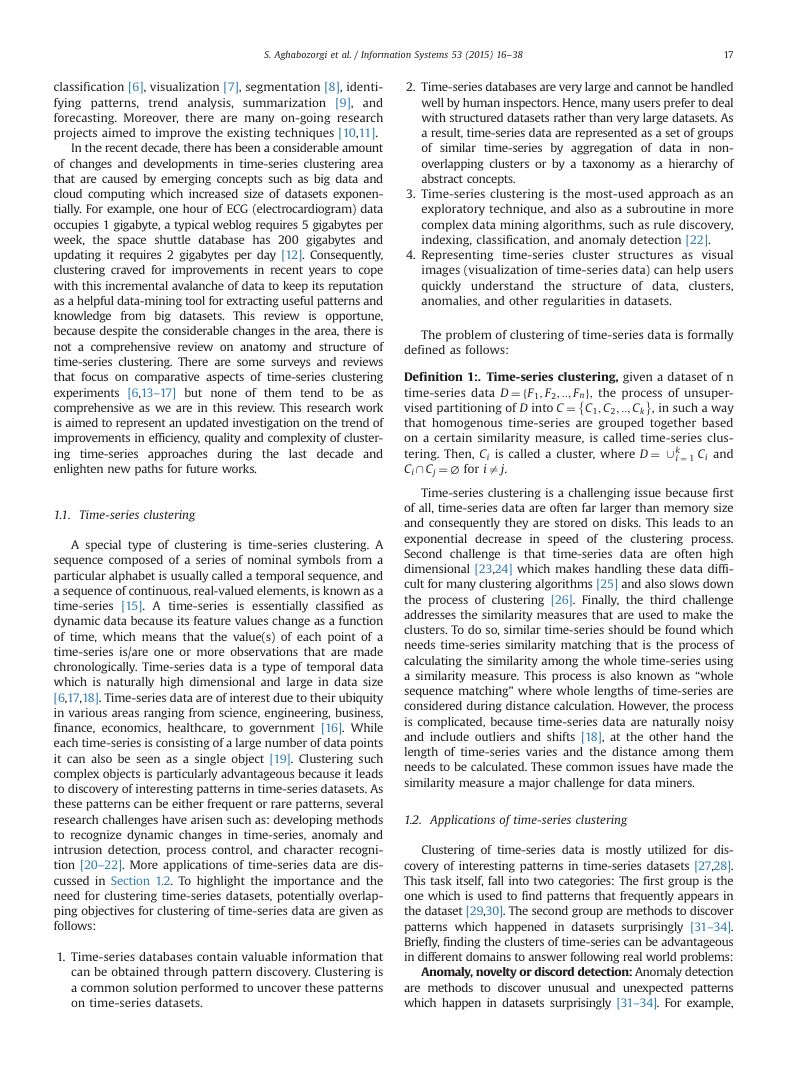
Fig. 1. Time-series clustering taxonomy.
1.3. Taxonomy of time-series clustering
Reviewing the literature, one can conclude that most of
clustering time-series related works are classified into three
categories: “whole time-series clustering”, “subsequence clus-
tering” and “time point clustering” as depicted in Fig. 1. The
first two categories are mentioned by Keogh and Lin [242] On
behalf of Ali Shirkhorshidi (shirkhorshidi_ali@yahoo.co.uk).
� Whole time-series clustering is considered as cluster-
ing of a set of individual time-series with respect to their
similarity. Here, clustering means applying conventional
�
S. Aghabozorgi et al. / Information Systems 53 (2015) 16–38
19
(usually) clustering on discrete objects, where objects
are time-series.
� Subsequence clustering means clustering on a set of
subsequences of a time-series that are extracted via a
sliding window, that is, clustering of segments from a
single long time-series.
� Time point clustering is another category of clustering
which is seen in some papers [74–76]. It is clustering of
time points based on a combination of their temporal
proximity of time points and the similarity of the corre-
sponding values. This approach is similar to time-series
segmentation. However, it is different from segmentation
as all points do not need to be assigned to clusters, i.e.,
some of them are considered as noise.
Essentially, sub-sequence clustering is performed on a
single time-series, and Keogh and Lin [242] represented that
this type of clustering is meaningless. Time-point clustering
also is applied on a single time-series, and is similar to time-
series segmentation as the objective of time-point clustering
is finding the clusters of time-point instead of clusters of
time-series data. The focus of this study is on the “whole
time-series clustering”. A complete review on whole time-
series clustering is performed and shown in Table 4. Review-
ing the literature, it is noticeable that various techniques have
been recommended for the clustering of whole time-series
data. However, most of them take one of the following
approaches to cluster time-series data:
1. Customizing the existing conventional clustering algorithms
(which work with static data) such that they become
compatible with the nature of time-series data. In this
approach, usually their distance measure (in conventional
algorithms) is modified to be compatible with the raw time-
series data [16].
2. Converting time-series data into simple objects (static
data) as input of conventional clustering algorithms [16].
3. Using multi resolutions of time-series as input of a
multi-step approach. This approach is discussed further
in Section 5.6.
Beside this common characteristic, there are generally
three different ways to cluster time-series, namely shape-
based, feature-based and model-based.
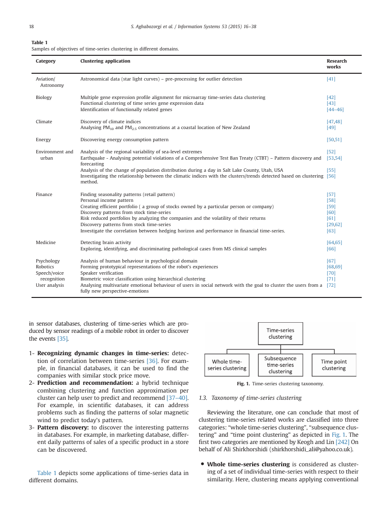
Fig. 2 shows a brief of these approaches. In the shape-
based approach, shapes of two time-series are matched as
well as possible, by a non-linear stretching and contracting
of the time axes. This approach has also been labelled as a
raw-data-based approach because it typically works directly
with the raw time-series data. Shape-based algorithms
usually employ conventional clustering methods, which
are compatible with static data while their distance/simi-
larity measure has been modified with an appropriate one
for time-series. In the feature-based approach, the raw
time-series are converted into a feature vector of lower
dimension. Later, a conventional clustering algorithm is
applied to the extracted feature vectors. Usually in this
approach, an equal length feature vector is calculated from
each time-series followed by the Euclidean distance mea-
surement [77]. In model-based methods, a raw time-series
is transformed into model parameters (a parametric model
Fig. 2. The time-series clustering approaches.
�
20
S. Aghabozorgi et al. / Information Systems 53 (2015) 16–38
time-series to a lower dimensional space or by feature
extraction. The reason that dimensionality reduction is
greatly important in clustering of time-series is firstly because
it reduces memory requirements as all raw time-series
cannot fit in the main memory [9,24]. Secondly, distance
calculation among raw data is computationally expensive,
and dimensionality reduction significantly speeds up cluster-
ing [9,24]. Finally, when measuring the distance between two
raw time-series, highly unintuitive results may be garnered,
because some distance measures are highly sensitive to some
“distortions” in the data [3,83], and consequently, by using
raw time-series, one may cluster time-series which are
similar in noise instead of clustering them based on similarity
in shape. The potential to obtain a different type of cluster is
the reason why choosing the appropriate approach for
dimension reduction (feature extraction) and its ratio is a
challenging task [26]. In fact, it is a trade-off between speed
and quality and all efforts must be made to obtain a proper
balance point between quality and execution time.
�
Definition 2:. Time-series representation, given a time-
series data Fi ¼ f 1; ::; f t; ::; f T
, representation is transform-
ing the time-series to another dimensionality reduced
where xoT and if two series are
vector F'
similar in the original space, then their representations
should be similar in the transformation space too.
n
i ¼ f '
o
1; ::; f '
x
According to [83], choosing an appropriate data representa-
tion method can be considered as the key component which
effects the efficiency and accuracy of the solution. High
dimensionality and noise are characteristics of most time-
series data [6], consequently, dimensionality reduction meth-
ods are usually used in whole time-series clustering in order to
address these issues and promote the performance. Time-
series dimensionality reduction techniques have progressed a
long way and are widely used with large scale time-series
dataset and each has its own features and drawbacks. Accord-
ingly, many researches had been carried out focusing on
representation and dimensionality reduction [84–90]. It is
worth here to mention about the one of the recent compar-
isons on representation methods. H. Ding et al. [91] have
performed a comprehensive comparison of 8 representation
methods on 38 datasets. Although, they had investigated the
indexing effectiveness of representation methods, the results
are advantageous for clustering purpose as well. They use
tightness of lower bounds to compare representation methods.
They show that there is very little difference between recent
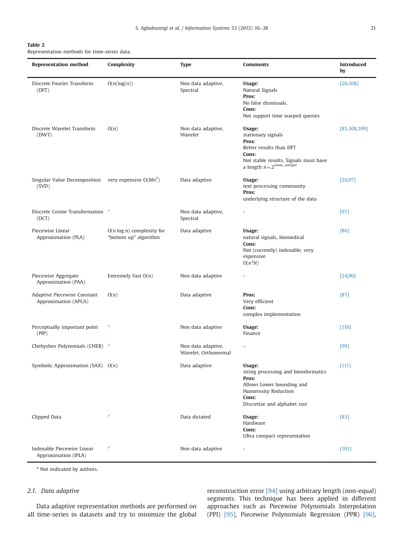
representation methods. In taxonomy of representations, there
are generally four representation types [9,83,92,93]: data
adaptive, non-data adaptive, model-based and data dictated
representation approaches as are depicted in Fig. 4.
Fig. 4. Hierarchy of different time-series representation approaches.
Fig. 3. An overview of four components of whole time-series clustering.
for each time-series,) and then a suitable model distance
and a clustering algorithm (usually conventional clustering
algorithms) is chosen and applied to the extracted model
parameters [16]. However, it is shown that usually model-
based approaches has scalability problems [78], and its
performance reduces when the clusters are close to each
other [79].
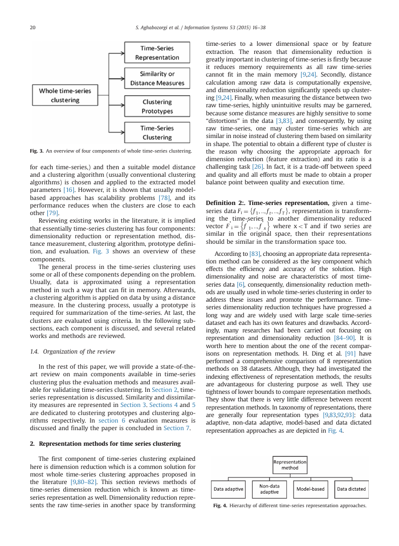
Reviewing existing works in the literature, it is implied
that essentially time-series clustering has four components:
dimensionality reduction or representation method, dis-
tance measurement, clustering algorithm, prototype defini-
tion, and evaluation. Fig. 3 shows an overview of these
components.
The general process in the time-series clustering uses
some or all of these components depending on the problem.
Usually, data is approximated using a representation
method in such a way that can fit in memory. Afterwards,
a clustering algorithm is applied on data by using a distance
measure. In the clustering process, usually a prototype is
required for summarization of the time-series. At last, the
clusters are evaluated using criteria. In the following sub-
sections, each component is discussed, and several related
works and methods are reviewed.
1.4. Organization of the review
In the rest of this paper, we will provide a state-of-the-
art review on main components available in time-series
clustering plus the evaluation methods and measures avail-
able for validating time-series clustering. In Section 2, time-
series representation is discussed. Similarity and dissimilar-
ity measures are represented in Section 3. Sections 4 and 5
are dedicated to clustering prototypes and clustering algo-
rithms respectively. In section 6 evaluation measures is
discussed and finally the paper is concluded in Section 7.
2. Representation methods for time series clustering
The first component of time-series clustering explained
here is dimension reduction which is a common solution for
most whole time-series clustering approaches proposed in
the literature [9,80–82]. This section reviews methods of
time-series dimension reduction which is known as time-
series representation as well. Dimensionality reduction repre-
sents the raw time-series in another space by transforming
�
S. Aghabozorgi et al. / Information Systems 53 (2015) 16–38
21
Introduced
by
[20,108]
[85,108,109]
[20,97]
[97]
[86]
[24,90]
[87]
[110]
[99]
[111]
[83]
[101]
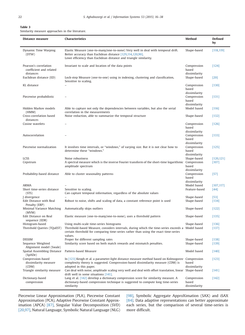
Table 2
Representation methods for time-series data.
Representation method
Complexity
Type
Comments
Discrete Fourier Transform
O(n(log(n))
(DFT)
Non data adaptive,
Spectral
Discrete Wavelet Transform
O(n)
(DWT)
Non data adaptive,
Wavelet
Singular Value Decomposition
very expensive O(Mn2)
Data adaptive
(SVD)
Usage:
Natural Signals
Pros:
No false dismissals.
Cons:
Not support time warped queries
Usage:
stationary signals
Pros:
Better results than DFT
Cons:
Not stable results, Signals must have
a length n¼2some_integer
Usage:
text processing community
Pros:
underlying structure of the data
Discrete Cosine Transformation
a
(DCT)
Non data adaptive,
Spectral
-
Piecewise Linear
Approximation (PLA)
O(n log n) complexity for
“bottom up” algorithm
Data adaptive
Usage:
natural signals, biomedical
Cons:
Not (currently) indexable, very
expensive
O(n2N)
Piecewise Aggregate
Approximation (PAA)
Extremely Fast O(n)
Non data adaptive
-
Adaptive Piecewise Constant
O(n)
Approximation (APCA)
Data adaptive
Pros:
Very efficient
Cons:
complex implementation
Perceptually important point
(PIP)
Chebyshev Polynomials (CHEB)
a
a
Non data adaptive
Usage:
Finance
Non data adaptive,
Wavelet, Orthonormal
–
Symbolic Approximation (SAX) O(n)
Data adaptive
Usage:
string processing and bioinformatics
Pros:
Allows Lower bounding and
Numerosity Reduction
Cons:
Discretize and alphabet size
Usage:
Hardware
Cons:
Ultra compact representation
Data dictated
Non data adaptive
-
a
a
Clipped Data
Indexable Piecewise Linear
Approximation (IPLA)
a Not indicated by authors.
2.1. Data adaptive
Data adaptive representation methods are performed on
all time-series in datasets and try to minimize the global
reconstruction error [94] using arbitrary length (non-equal)
segments. This technique has been applied in different
approaches such as Piecewise Polynomials Interpolation
(PPI) [95], Piecewise Polynomials Regression (PPR) [96],
�
22
S. Aghabozorgi et al. / Information Systems 53 (2015) 16–38
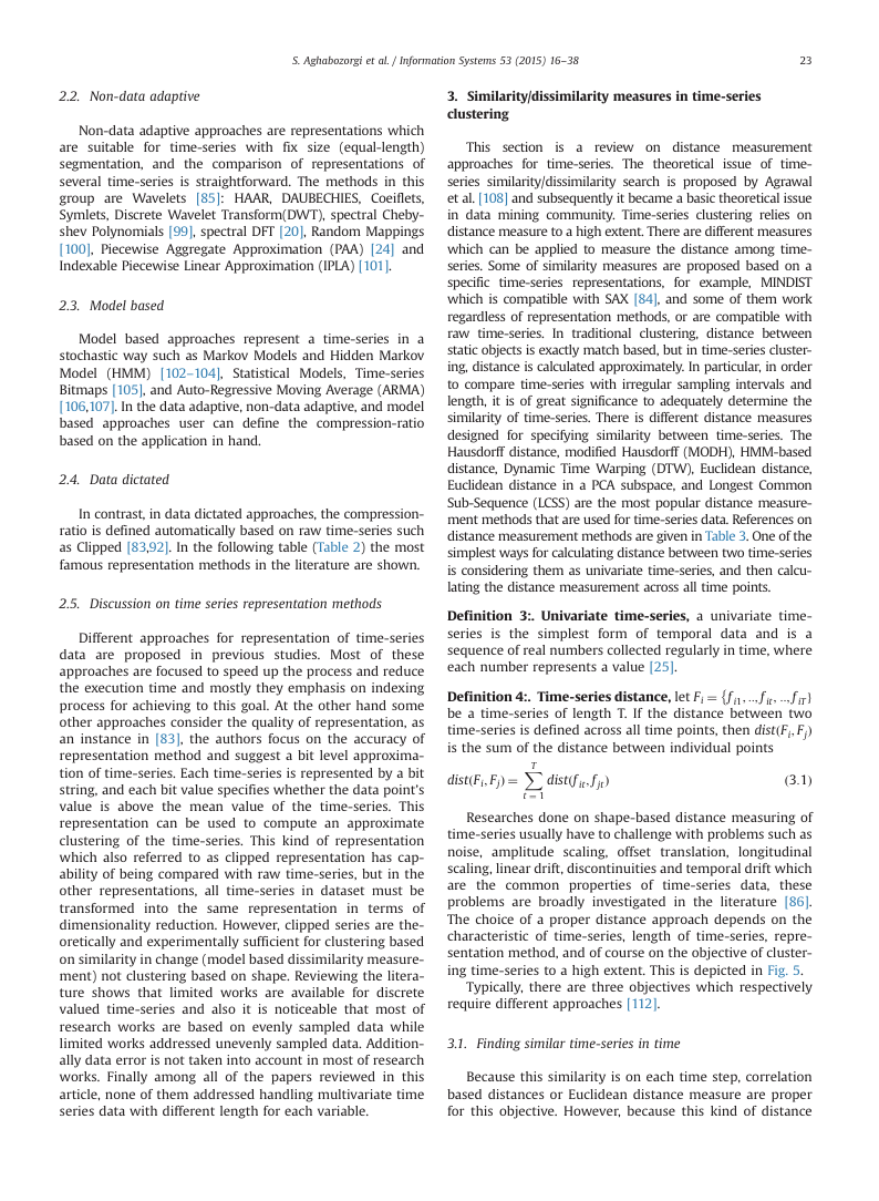
Table 3
Similarity measure approaches in the literature.
Distance measure
Characteristics
Dynamic Time Warping
(DTW)
Elastic Measure (one-to-many/one-to-none) Very well in deal with temporal drift.
Better accuracy than Euclidean distance [129,114,120,90].
Lowe efficiency than Euclidean distance and triangle similarity.
Pearson’s correlation
coefficient and related
distances
Euclidean distance (ED)
KL distance
Invariant to scale and location of the data points
Lock-step Measure (one-to-one) using in indexing, clustering and classification,
Sensitive to scaling.
–
Piecewise probabilistic
–
Hidden Markov models
(HMM)
Cross-correlation based
distances
Cosine wavelets
Autocorrelation
Able to capture not only the dependencies between variables, but also the serial
correlation in the measurements
Noise reduction, able to summarize the temporal structure
–
–
Piecewise normalization
It involves time intervals, or “windows,” of varying size. But it is not clear how to
determine these “windows.”
LCSS
Cepstrum
Noise robustness
A spectral measure which is the inverse Fourier transform of the short-time logarithmic
amplitude spectrum
Probability-based distance
Able to cluster seasonality patterns
ARMA
Short time-series distance
(STS)
J divergence
Edit Distance with Real
Penalty (ERP)
–
Sensitive to scaling.
Can capture temporal information, regardless of the absolute values
–
Robust to noise, shifts and scaling of data, a constant reference point is used
Minimal Variance Matching
Automatically skips outliers
(MVM)
Edit Distance on Real
Elastic measure (one-to-many/one-to-none), uses a threshold pattern
Method
Defined
by
Shape-based
[118,119]
Compression
based
dissimilarity
Shape-based
Compression
based
dissimilarity
Compression
based
dissimilarity
Model based
Shape-based
Compression
based
dissimilarity
Compression
based
dissimilarity
Compression
based
dissimilarity
Shape-based
Compression
based
dissimilarity
Compression
based
dissimilarity
Model based
Feature-based
Shape-based
Shape-based
Shape-based
Shape-based
Shape-based
Model based
Shape-based
Shape-based
Model based
[124]
[20]
[130]
[131]
[116]
[132]
[126]
[133]
[125]
[120,121]
[107]
[57]
[107,117]
[44]
[53]
[134]
[122]
[135]
[136]
[137]
[138]
[139]
[140]
[123]
[141]
[142]
sequence (EDR)
Histogram-based
Threshold Queries (TQuEST)
DISSIM
Sequence Weighted
Alignment model (Swale)
Spatial Assembling Distance
(SpADe)
Compression-based
dissimilarity measure
(CDM)
Triangle similarity measure
Dictionary-based
compression
Using multi-scale time-series histograms
Threshold-based Measure, considers intervals, during which the time-series exceeds a
certain threshold for comparing time-series rather than using the exact time-series
values.
Proper for different sampling rates
Similarity score based on both match rewards and mismatch penalties.
Pattern-based Measure
In [123] Keogh et al. a parameter-light distance measure method based on Kolmogorov
complexity theory is suggested. Compression-based dissimilarity measure (CDM) is
adopted in this paper.
Can deal with noise, amplitude scaling very well and deal with offset translation, linear
drift well in some situations [141].
Lang et al. [142] develop a dictionary compression score for similarity measure. A
dictionary-based compression technique is suggested to compute long time-series
similarity
Compression
based
dissimilarity
Shape-based
Compression
based
dissimilarity
Piecewise Linear Approximation (PLA), Piecewise Constant
Approximation (PCA), Adaptive Piecewise Constant Approx-
imation (APCA) [87], Singular Value Decomposition (SVD)
[20,97], Natural Language, Symbolic Natural Language (NLG)
[98], Symbolic Aggregate ApproXimation (SAX) and iSAX
[84]. Data adaptive representations can better approximate
each series, but the comparison of several time-series is
more difficult.
�
S. Aghabozorgi et al. / Information Systems 53 (2015) 16–38
23
2.2. Non-data adaptive
Non-data adaptive approaches are representations which
are suitable for time-series with fix size (equal-length)
segmentation, and the comparison of representations of
several time-series is straightforward. The methods in this
group are Wavelets [85]: HAAR, DAUBECHIES, Coeiflets,
Symlets, Discrete Wavelet Transform(DWT), spectral Cheby-
shev Polynomials [99], spectral DFT [20], Random Mappings
[100], Piecewise Aggregate Approximation (PAA) [24] and
Indexable Piecewise Linear Approximation (IPLA) [101].
2.3. Model based
(HMM)
Model based approaches represent a time-series in a
stochastic way such as Markov Models and Hidden Markov
Model
[102–104], Statistical Models, Time-series
Bitmaps [105], and Auto-Regressive Moving Average (ARMA)
[106,107]. In the data adaptive, non-data adaptive, and model
based approaches user can define the compression-ratio
based on the application in hand.
2.4. Data dictated
In contrast, in data dictated approaches, the compression-
ratio is defined automatically based on raw time-series such
as Clipped [83,92]. In the following table (Table 2) the most
famous representation methods in the literature are shown.
2.5. Discussion on time series representation methods
Different approaches for representation of time-series
data are proposed in previous studies. Most of these
approaches are focused to speed up the process and reduce
the execution time and mostly they emphasis on indexing
process for achieving to this goal. At the other hand some
other approaches consider the quality of representation, as
an instance in [83], the authors focus on the accuracy of
representation method and suggest a bit level approxima-
tion of time-series. Each time-series is represented by a bit
string, and each bit value specifies whether the data point’s
value is above the mean value of the time-series. This
representation can be used to compute an approximate
clustering of the time-series. This kind of representation
which also referred to as clipped representation has cap-
ability of being compared with raw time-series, but in the
other representations, all time-series in dataset must be
transformed into the same representation in terms of
dimensionality reduction. However, clipped series are the-
oretically and experimentally sufficient for clustering based
on similarity in change (model based dissimilarity measure-
ment) not clustering based on shape. Reviewing the litera-
ture shows that limited works are available for discrete
valued time-series and also it is noticeable that most of
research works are based on evenly sampled data while
limited works addressed unevenly sampled data. Addition-
ally data error is not taken into account in most of research
works. Finally among all of the papers reviewed in this
article, none of them addressed handling multivariate time
series data with different length for each variable.
3. Similarity/dissimilarity measures in time-series
clustering
This
section is a review on distance measurement
approaches for time-series. The theoretical
issue of time-
series similarity/dissimilarity search is proposed by Agrawal
et al. [108] and subsequently it became a basic theoretical issue
in data mining community. Time-series clustering relies on
distance measure to a high extent. There are different measures
which can be applied to measure the distance among time-
series. Some of similarity measures are proposed based on a
specific time-series representations,
for example, MINDIST
which is compatible with SAX [84], and some of them work
regardless of representation methods, or are compatible with
raw time-series. In traditional clustering, distance between
static objects is exactly match based, but in time-series cluster-
ing, distance is calculated approximately. In particular, in order
to compare time-series with irregular sampling intervals and
length, it is of great significance to adequately determine the
similarity of time-series. There is different distance measures
designed for specifying similarity between time-series. The
Hausdorff distance, modified Hausdorff (MODH), HMM-based
distance, Dynamic Time Warping (DTW), Euclidean distance,
Euclidean distance in a PCA subspace, and Longest Common
Sub-Sequence (LCSS) are the most popular distance measure-
ment methods that are used for time-series data. References on
distance measurement methods are given in Table 3. One of the
simplest ways for calculating distance between two time-series
is considering them as univariate time-series, and then calcu-
lating the distance measurement across all time points.
Definition 3:. Univariate time-series, a univariate time-
series is the simplest form of temporal data and is a
sequence of real numbers collected regularly in time, where
each number represents a value [25].
Definition 4:. Time-series distance, let Fi ¼ f i1; ::; f it;
::; f iTg
be a time-series of length T. If the distance between two
time-series is defined across all time points, then distðFi; FjÞ
is the sum of the distance between individual points
distðFi; FjÞ ¼
distðf it; f jtÞ
ð3:1Þ
�
XT
t ¼ 1
Researches done on shape-based distance measuring of
time-series usually have to challenge with problems such as
noise, amplitude scaling, offset translation,
longitudinal
scaling, linear drift, discontinuities and temporal drift which
are the common properties of time-series data, these
problems are broadly investigated in the literature [86].
The choice of a proper distance approach depends on the
characteristic of time-series, length of time-series, repre-
sentation method, and of course on the objective of cluster-
ing time-series to a high extent. This is depicted in Fig. 5.
Typically, there are three objectives which respectively
require different approaches [112].
3.1. Finding similar time-series in time
Because this similarity is on each time step, correlation
based distances or Euclidean distance measure are proper
for this objective. However, because this kind of distance
�


 2023年江西萍乡中考道德与法治真题及答案.doc
 2012年重庆南川中考生物真题及答案.doc
 2013年江西师范大学地理学综合及文艺理论基础考研真题.doc
 2020年四川甘孜小升初语文真题及答案I卷.doc
 2020年注册岩土工程师专业基础考试真题及答案.doc
 2023-2024学年福建省厦门市九年级上学期数学月考试题及答案.doc
 2021-2022学年辽宁省沈阳市大东区九年级上学期语文期末试题及答案.doc
 2022-2023学年北京东城区初三第一学期物理期末试卷及答案.doc
 2018上半年江西教师资格初中地理学科知识与教学能力真题及答案.doc
 2012年河北国家公务员申论考试真题及答案-省级.doc
 2020-2021学年江苏省扬州市江都区邵樊片九年级上学期数学第一次质量检测试题及答案.doc
 2022下半年黑龙江教师资格证中学综合素质真题及答案.doc