Adaptive detection and parameter estimation for multidimensional....pdf-资料库

MASSACHUSETTS INSTITUTE OF TECHNOLOGY LINCOLN LABORATORY ADAPTIVE DETECTION AND PARAMETER ESTIMATION FOR MULTIDIMENSIONAL SIGNAL MODELS E.J. KELLY Group 61 X.M. FORSYTHE Group 44 copy '/ I TECHNICAL REPORT "84 , i " ' ... . ; i . .. . . . . 19 APRIL 1989.. Approved for public release; distribution is unlimited. LEXINGTON MASSACHUSETTS

"ABSTRACT The problem of target detection and signal parameter estimation in a background of unknown interference is studied, using a multidimen- sional generalization of the signal models usually employed for radar, sonar, and similar applications The required techniques of multivariate statistical _a:lysis are developed and extensively used throughout the stud:, and the necessary mathematical background is provided in Appendices. Target detection performance is shown to be governed by a form of the Wilks' Lambda statistic, and a new method for its numeri- cal evaluation is given which applies to the probability of false alarm of the detector. Signal parameter estimation is shown to be directly related to known techniques of adaptive nulling, and several new results rele- vant to adaptive nulling performance are obtained. Ill

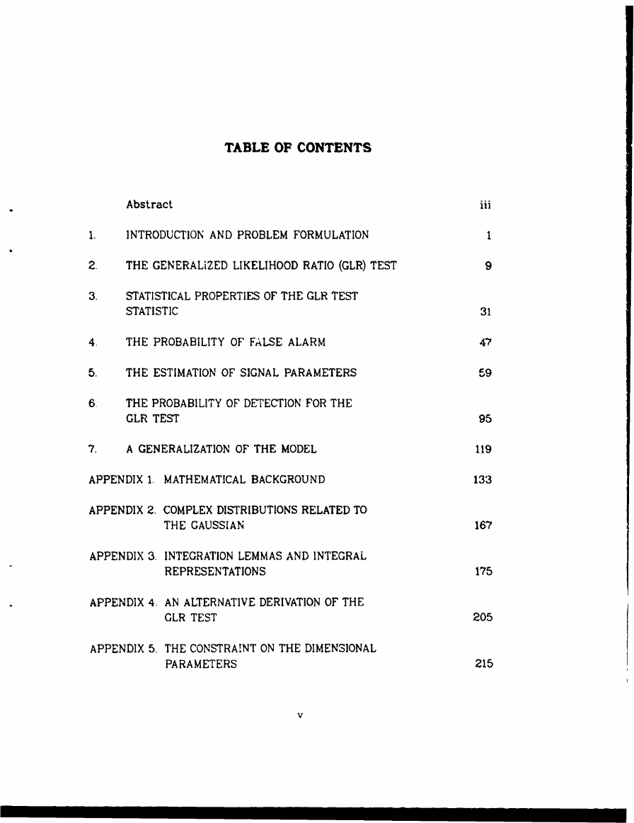
TABLE OF CONTENTS Abstract INTRODUCTION AND PROBLEM FORMULATION THE GENERALIZED LIKELIHOOD RATIO (GLR) TEST STATISTICAL PROPERTIES OF THE GLR TEST STATISTIC THE PROBABILITY OF FALSE ALARM THE ESTIMATION OF SIGNAL PARAMETERS THE PROBABILITY OF DETECTION FOR THE GLR TEST 1. 2. 3. 4. 5. 6. 7. A GENERALIZATION OF THE MODEL APPENDIX 1. MATHEMATICAL BACKGROUND APPENDIX 2. COMPLEX DISTRIBUTIONS RELATED TO THE GAUSSIAN APPENDIX 3. INTEGRATION LEMMAS AND INTEGRAL REPRESENTATIONS APPENDIX 4. AN ALTERNATIVE DERIVATION OF THE GLR TEST APPENDIX 5. THE CONSTRAINT ON THE DIMENSIONAL PARAMETERS V iii 1 9 31 47 59 95 119 133 167 175 205 215

APPENDIX 6. NUMERICAL COMPUTATION OF THE FALSE ALARM PROBABILITY APPENDIX 7. COMPUTATIONAL ALGORITHMS REFERENCES 221 233 241 vi

1. INTRODUCTION AND PROBLEM FORMULATION The basic physical model which motivates this study corresponds to an array of sensors of some kind, positioned in an arbitrary way in space, and providing inputs to a processor whose nature is the subject of the analysis. One "sample" is a set of out- puts from this array, arranged as a vector. These samples may come directly from the elements of the array, or they may be the outputs from a beamforming network of some kind. We use complex variables to represent the data since we are concerned with signals which modulate a carrier. Then the real and imaginary parts of a com- plex quantity represent the in-phase and quadrature components of such a signal. The modifications required to deal with real data are generally straightforward. The basic data set upon which a processor will operate is a collection of sample vectors, arranged as the columns of a rectangular data array. We do not wish to specify the physical arrangements in greater detail because the mathematical model itself is applicable to many diverse systems which may use adaptive processing of array outputs in the radar, optical, and acoustical fields, and so on Indeed, the ele- ments of the sample vectors could easily have a significance other than the direct outputs of some set of sensors. However, we wish to draw etl.ention to certain basic assumptions made in our model which, in certain cases, will limit its relevance. We model the data array as a set of Gaussian random variables, and the covari- ance structure of the modei is used to characterize the "noise" component of the data, including both system noise and any random external interference. On the other hand, "signals" are considered to be more structured contributions to the input, and these are modeled by making appropriate assumptions about the mean values of the elements of the data array. The emphasis here is on the detection of these signals and the estimation of their parameters, and the most natural applications are to radar or active sonar, where coherent processing is possible due to the known form of the signals. In this study, a general linear model is used to represent signals. Our strongest assumption concerning the covariance structure is a postulate of stationarity: the sample vectors are assumed to be statistically independent and to share a common covariance rmatrix. If the samples correspond to successive times, then this is stationarity in the usual sense. However, the concept can be applied in other ways. Fbr example, in the iadar case the samples may correspond to successive range bins; but the data may already have been subjected to some form of processing embracing a larger interval of time, such as Fourier transformation (Doppler process- ing) of the array outputs before the adaptive phase of the process in which we are interested. I II II I I r I ll i ' i _i .n a I .1

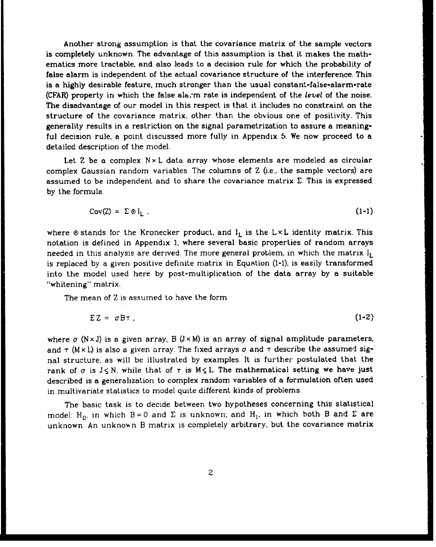
Another strong assumption is that the covariance matrix of the sample vectors is completely unknown. The advantage of this assumption is that it makes the math- ematics more tractable, and also leads to a decision rule for which the probability of false alarm is independent of the actual covariance structure of the interference. This is a highly desirable feature, much stronger than the usual constant-false-alarm-rate (CFAR) property in which the false alarm rate is independent of the level of the noise. The disadvantage of our model in this respect is that it includes no constraint on the structure of the covariance matrix, other than the obvious one of positivity. This generality results in a restriction on the signal parametrization to assure a meaning- ful decision rule, a point discussed more fully in Appendix 5. We now proceed to a detailed description of the model. Let Z be a complex N x L data array whose elements are modeled as circular complex Gaussian random variables. The columns of Z (i.e., the sample vectors) are assumed to be independent and to share the covariance matrix S. This is expressed by the formula Cov(Z) = e I-) where ® stands for the Kronecker product, and IL is the L x L identity matrix. This notation is defined in Appendix I. where several basic properties of random arrays needed in this analysis are derived The more general problem, in which the matrix IL is replaced by a given positive definite matrix in Equation (1-I). is easily transformed into the model used here by post-multiplication of the data array by a suitable "whitening" matrix. The mean of Z is assumed to have the form EZ = aBT, (,-2) where a (N x J) is a given array, B (J x M) is an array of signal amplitude parameters, and T- (M x L) is also a given array. The fixed arrays a and T describe the assumed sig- nal structure, as will be illustrated by examples. 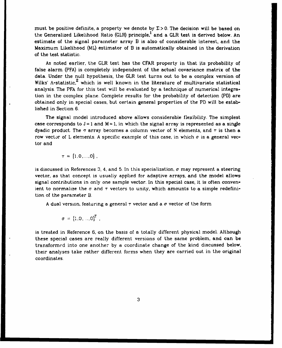It is further postulated that the rank of a is Jmust be positive definite, a property we denote by E > 0. The decision will be based on the Generalized Likelihood Ratio (GLR) principle,. and a GLR test is derived below. An estimate of the signal parameter array B is also of considerable interest, and the Maximum Likelihood (ML) estimator of B is automatically obtained in the derivation of the test statistic. As noted earlier, the GLR test has the CFAR property in that its probability of false alarm (PFA) is completely independent of the actual covariance matrix of the data. Under the null hypothesis, the GLR test turns out to be a complex version of Wilks' A-statistic,2 which is well known in the literature of multivariate statistical analysis. The PFA for this test will be evaluated by a technique of numerical integra- tion in the complex plane. Complete results for the probability of detection (PD) are obtained only in special cases, but certain general properties of the PD will be estab- lished in Section 6. The signal model introduced above allows considerable flexibility. The simplest case corresponds to J = 1 and M = 1, in which the signal array is represented as a single dyadic product. The T array becomes a column vector of N elements, and T is then a row vector of L elements. A specific example of this case, in which a is a general vec- tor and r dl,O....0], is discussed in References 3, 4, and 5. In this specialization, a may represent a steering vector, as that concept is usualiy applied for adaptive arrays, and the model allows signal contributions in only one sample vector. In this special case, it is often conven- ient to normalize the a and T vectors to unity, which amounts to a simple redefini- tion of the parameter B. A dual version, featuring a general T vector and a a vector of the form o : i. .. _ 0 1T is treated in Reference 6, on the basis of a totally different physical model, Although these special cases are really different versions of the same problem, and can be transformed into one another by a coordinate change of the kind discussed below, their analyses take rather different forms when they are carried out in the original coordinates. 3
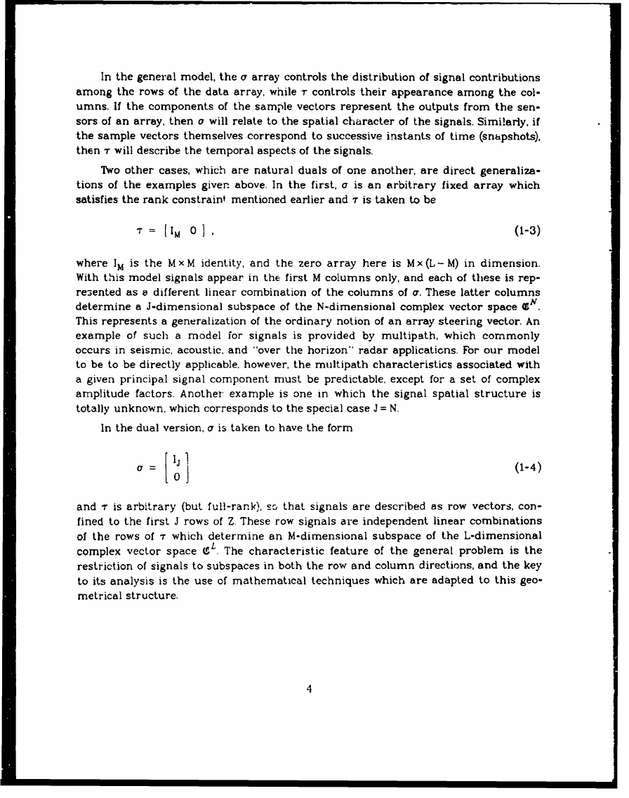
In the general model, the a array controls the distribution of signal contributions among the rows of the data array, while -r controls their appearance among the col- umns. If the components of the sample vectors represent the outputs from the sen- sors of an array, then a will relate to the spatial character of the signals. Similarly. if the sample vectors themselves correspond to successive instants of time (snapshots). then T will describe the temporal aspects of the signals. Two other cases, which are natural duals of one another, are direct generaliza- tions of the examples given above. In the first, a is an arbitrary fixed array which satisfies the rank constraint mentioned earlier and T is taken to be T- = [I 0 (1-3) where IM is the M x M identity, and the zero array here is M x (L - M) in dimension. With this model signals appear in the first M columns only, and each of these is rep- relented as a different linear combination of the columns of a. These latter columns determine a J-dimensional subspace of the N-dimensional complex vector space C This represents a generalization of the ordinary notion of an array steering vector. An example of such a model for signals is provided by multipath, which commonly occurs in seismic, acoustic, and "over the horizon" radar applications. For our model to be to be directly applicable, however, the multipath characteristics associated with a given principal signal component must be predictable, except for a set of complex amplitude factors. Another example is one in which the signal spatial structure is totally unknown, which corresponds to the special case J = N. In the dual version, a is taken to have the form Ij! a= (1-4) and Tr is arbitrary (but full-rank), sc that signals are described as row vectors, con- fined to the first J rows of Z. These row signals are independent linear combinations of the rows of T which determine an M-dimensional subspace of the L-dimensional complex vector space eL. The characteristic feature of the general problem is the restriction of signals to subspaces in both the row and column directions, and the key to its analysis is the use of mathematical techniques which are adapted to this geo- metrical structure. 4

资料库

Adaptive detection and parameter estimation for multidimensional....pdf

相关推荐

行业

热门标签

最新资料