IEEE TRANSACTIONS ON ACOUSTICS, SPEECH, AND SIGNAL PROCESSING, VOL. ASSP-29, NO. 3, JUNE 1981 571
has also included the application of digital signal processing to acoustic
signature simulation and the system design of large scale digital sonars.
He is presently working toward the Ph.D. degree in electrical engineer-
ing at the University of Southern California under a Hughes Aircraft
Company fellowship.
Paul L. Feintuch (SY66-M’67)
received the
B.S.E.E. degree from the Cooper Union, New
York, NY, in 1967, and the M.S.E.E. and Ph.D.
degrees in electrical engineering from the Uni-
versity of Southern California, Los Angeles, in
1969 and 1972, respectively.
He is
currently with the
Company, Fullerton, CA, where he
Scientist in the
primary interest in research and development in
all aspects of sonar signal processing and in the
Systems Laboratory, with
Hughes Aircraft
is Senior
Neil J. Bershad (S’60-M’62) was born in Brook-
lyn, NY, on October 20, 1937. He received the
B.E.E. degree from Rensselaer Polytechnic
Institute, Troy, NY, in 1958, the M.S. degree
in electrical engineering from the University of
Southern California, Los Angeles, in 1960, and
the Ph.D. degree in electrical engineering from
Rensselaer Polytechnic Institute in 1962.
In 1966 he joined the Faculty of the School
of Engineering, University of California, Irvine,
where he is now a Professor of Electrical En-
gineering. His research interests have involved stochastic system model-
ing and analysis. His present interests are in the areas of detection and
estimation using multiple observations, and the
statistical behavior of
five years,
nonlinear systems driven by stochastic inputs. For the past
he has served as an Associate Editor of the IEEE TRANSACTIONS
ON COM-
MUNICATIONS in the area of phase-locked loops and synchronization. He
is presently a Consultant in array processing to the Hughes Aircraft Com-
pany, Fullerton, CA.
Time Delay Estimation Using the LMS Adaptive
Filter-Dynamic Behavior
Abstract-The LMS adaptive filter is used to estimate a Linearly mov-
ing time delay between two broad-band waveforms. The tracking be-
havior of the mean weights is analyzed and is compared with simula-
tions of the actual device.
T
I. INTRODUCTION
HE concept of using an LMS adaptive filter, configured as
a canceller to estimate the time delay difference between
two waveforms, is studied in [ l ] for a static time delay. The
estimate of delay is obtained by interpolating on the weights
in the filter to select the point in the tapped delay line that
Manuscript received May 9, 1980; revised September 30,1980. This
work was supported by the Naval Sea Systems Command Code 63R
under Contract N00024-77-C-6251.
P. L. Feintuch and F. A. Reed are with Hughes Aircraft Company,
Fullerton, CA 92634.
N. J. Bershad is with the Department of Electrical Engineering, Uni-
versity of California, Irvine, CA 92664, and is a consultant to Hughes
Aircraft Company, Fullerton, CA 92634.
corresponds to the peak weight. The resulting estimate is un-
biased in the nonmoving input case, and the variance is within
0.5 dB of the Cram&-Rao lower bound for the variance of any
delay estimate using the same data. In addition, it was shown
that if assumed a priori statistics concerning the input power
spectra differ from what is actually the case, then the adaptive
filter tracker can dramatically outperform a fixed parameter
conventional tracker being operated in an environment other
than that‘for which it was designed.
Since the delay estimation is performed on the peak value of
the weights in the adaptive filter, the time constant for the se-
lection of the peak is the significant transient response. The
peak weight can be correctly selected much more quickly than
the time required for either the weights or the mean square er-
ror to converge [l] . This suggests that this processor has the
potential to track rapidly changing time delays by just observ-
ing the peak weight move through the adaptive filter tapped
delay line.
0096-3518/81/0600-0571$00.75 0 1981 IEEE
�
572
IEEE TRANSACTIONS ON ACOUSTICS, SPEECH, AND SIGNAL PROCESSING, VOL. ASSP-29, NO. 3, JUNE 1981
+ =
Y
-
d ( n ) = S(nTs - r (nTs1) + n1 (nTs) ,
S (nTs1 +np(nTs)
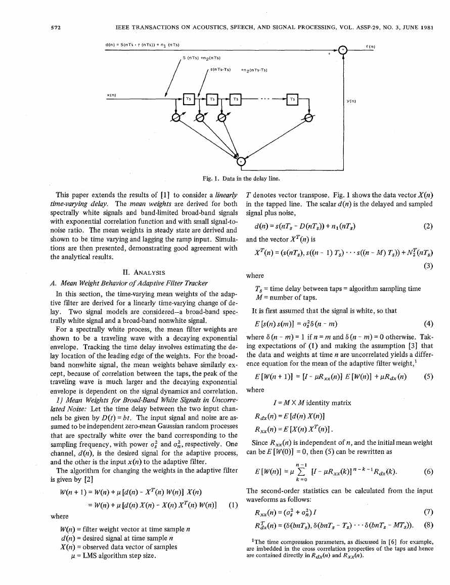
Fig. 1. Data in the delay line.
This paper extends the results of [l] to consider a linearly
time-varying delay. The mean weights are derived
for both
spectrally white signals and band-limited broad-band signals
with exponential correlation function and with small signal-to-
noise ratio. The mean weights in steady state are derived and
shown to be time varying and lagging the ramp input. Simula-
tions are then presented, demonstrating good agreement with
the analytical results.
A. Mean Weight Behavior of Adaptive Filter Tracker
11. ANALYSIS
In this section, the
time-varying mean weights of the adap-
tive filter are derived for a linearly time-varying change of de-
lay. Two signal models are considered-a
broad-band spec-
trally white signal and a broad-band nonwhite signal.
For a spectrally white process, the mean filter weights are
shown to be a traveling wave with a decaying exponential
envelope. Tracking the time delay involves estimating the de-
lay location of the leading edge of the weights. For the broad-
band nonwhite signal, the mean weights behave similarly ex-
cept, because of correlation between the taps, the peak of the
traveling wave is much larger and the decaying exponential
envelope is dependent on the signal dynamics and correlation.
I ) Mean Weights for Broad-Band White Signals in Uncorre-
lated Noise: Let the time delay between the two input chan-
nels be given by D(t) = bt. The input signal and noise are as-
sumed to be independent zero-mean Gaussian random processes
that are spectrally white over the band corresponding to the
sampling frequency, with power u,” and u i , respectively. One
channel, d(n), is the desired signal for the adaptive process,
and the other is the input x(n) to the adaptive filter.
The algorithm for changing the weights in the adaptive filter
is given by [2]
W(n t 1) = W(n) t p [d(n) - Xr(n) W(n)] X(n)
= W(n) t ~r [d(n) X(n) - X(n) XT(n) W(n)l
(1)
where
W(n) = filter weight vector at time sample n
d(n) = desired signal at time sample n
X(n) = observed data vector of samples
p = LMS algorithm step size.
T denotes vector transpose. Fig. 1 shows the data vector X(n)
in the tapped line. The scalar d(n) is the delayed and sampled
signal plus noise,
d(n) = s(nT, - D(nT,)) t nl(nT,)
(2)
and the vector XT(n) is
XT(n) = (s(nT,), s((n - 1) T,) * * s((n - M ) T,)) + N;f(nT,)
(3)
where
T, = time delay between taps = algorithm sampling time
M = number of taps.
It is first assumed that the signal is white, so that
E [s(n) s(m)J = u,”S(n - m)
(4)
where F (n - m) = 1 if n = m and 6 (n - m ) = 0 otherwise. Tak-
ing expectations of (1) and making the assumption [3] that
the data and weights at time n are uncorrelated yields a differ-
ence equation for the mean of the adaptive filter weight,’
E [W(n t 111 = [I - ruRxx(n)l E [W(n>l + PRdx(n)
(5)
where
I = M X M identity matrix
= E [d(n> Nn)1
Rxx(n) = E
Since R,(n)
XT(n)l *
is independent of n, and the initial mean weight
can be E [W(O)] = 0, then (5) can be rewritten as
E[W(n)J =pyl [ I - pRxx(k)]n-k-l dx (k).
(6)
k = O
The second-order statistics can be calculated from the input
waveforms as follows:
Rxx(n) = (u: t u i ) I
RTX(n) = (F(bnT,), G(bnT, - T,) . . . G(bnT, - MT,)).
(7)
(8)
‘The time compression parameters, as discussed in [ 6 ] for example,
are imbedded in the cross correlation properties of the taps and hence
are contained directly in Rdx(n) and Rxx(n).
�
FEINTUCH et al.: LMS ADAPTIVE FILTER-DYNAMIC BEHAVIOR
573
w,(n)
/l us*
0
. . . . . .
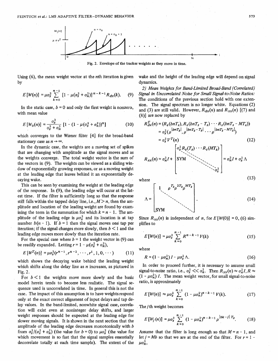
Fig. 2. Envelope of the tracker weights as they move in time.
I
N
) i
wake and the height of the leading edge will depend on signal
dynamics.
2) Mean Weights for Band-Limited Broad-Band (Correlated)
Signal in Uncorrelated Noise for Small Signal-to-Noise Ratios:
The conditions of the previous section hold with one exten-
sion. The signal spectrum is no longer white. Equations
(2)
and (3) are still valid. However, Rdx(n) and R,.(n) [(7) and
(S)] are now replaced by
RZx(n) = (R,(bnT,), R,(bnT, - T,) * - R,(bnT, - MT,))
10," R, (T,) - * R, (Mr,) 1
( 1 2)
lbnTsl
= 4 ( P
= a," VT(n)
, P
IbnTs- T,I
IbnTs-MTsl
" ' P
1
1
Since R,(n)
plifies to
is independent of n, for E [W(O)] = 0, (6) sim-
E[W(n)] =pa,"
n - 1
R n - k - l V
k=O
where
In order to proceed further, it is necessary to assume small
signal-to-noise ratio, i.e., u," << u i . Then R,(n) = air, R =
( 1 - pa;) I. The mean weight vector, for small signal-to-noise
ratio, is approximately
Using (6), the mean weight vector at the nth iteration is given
by
E[W(n)] =pus"
n - 1
k=O
[l - p(u," t u ; ) ] ~ - ~ - ' Rdx(k).
(9)
In the static case, b = 0 and only the first weight is nonzero,
with mean value
E [Wo(n)l =
0,"
as + on
[I - (1 - P(Q," +
( 1 0)
which converges to the Wiener filter [4] for the broad-band
stationary case as n + 00.
In the dynamic case, the weights are a moving set of spikes
that are changing with amplitude as the signal moves and as
the weights converge. The total weight vector is the sum of
the vectors in (9). The weights can be viewed as a sliding win-
dow of exponentially growing responses, or as a moving weight
at the leading edge that leaves behind it an exponentially de-
caying wake.
This can be seen by examining the weight at the leading edge
of the response. In (9), the leading edge will occur at the. lat-
est time. If the filter is sufficiently long so that the response
still falls within the tapped delay line, i.e.,M> n, then the am-
plitude and location of the leading weight are found by exam-
ining the term in the summation for which k = n - 1. The am-
plitude of the leading edge is p~," and its location is at tap
number b(n - 1). If b = 1 then the signal moves one tap per
iteration; if the signal changes more slowly, then b < 1 and the
leading edge moves more slowly than the iteration rate.
For the special case where b = 1 the weight vector in (9) can
be readily expanded. Letting r = 1 - p(u," t us),
E[WT(n)] =pa,"(rn-1,rn-2,...,r1,1,0,'..) (11)
which shows the decaying wake behind the leading weight
which shifts along the delay line as n increases, as pictured in
Fig. 2.
For b < 1 the weights move more slowly and the basic
model herein tends to become less realistic. The signal se-
quence used is uncorrelated in time. In general this is not the
case. The impact of this assumption is to have weights respond
only at the exact correct alignment of input delays and tap de-
lay values. In the band-limited, nonwhite signal case, correla-
tion will exist even at noninteger delay shifts, and larger
weight responses should be expected at the leading edge for
slower moving signals. It is shown in the next section that the
amplitude of the leading edge decreases monotonically with b
from o,"/(u,' t ai) (the value for b = 0) to pu," (the value for
which movement is so fast that the signal samples essentially
decorrelate totally at each time sample). The extent of the
�
5 74
IEEE TRANSACTIONS ON ACOUSTICS, SPEECH,
AND SIGNAL
PROCESSING, VOL.
ASSP-29, NO. 3, JUNE 1981
k=O
Equation (19) describes the transient behavior of the mean
weight for small signal-to-noise ratios. In steady state, i.e., M
arbitrarily large, one can readily see the relationships between
signal correlation p , signal dynamics b, and algorithm dynam-
ics p :
There are several cases of interest. If p = 1, then the signal is
totally correlated from tap to tap, regardless of signal dynam-
ics. For this case E [WMb(Oo)] = u:/o:.
This is a small signal-
to-noise ratio approximation to u,”/(ui + u;) which is what one
would expect in the static case. If p = 0, the signal is uncorre-
lated and again signal dynamics should not affect the result.
For this case, E[Wn/rb(””)] = pa: which agrees with (1 1) where
dynamics tended to decorrelate the signal. If there are no sig-
nal dynamics, Le., b = 0, then E [WMb (w)] = O:/O~
indepen-
dent of p, which is again the expected small signal-to-noise ra-
tio static
result. The tradeoff between dynamics and signal
correlation can be seen by examining the term pbTS in the ex-
pression for E[W&fb(w)] . As b decreases, pbTS looks more like
unity and the signal looks more correlated. As b increases, p
(which is less than one) is raised to a higher power and the sig-
nal has become less correlated.
B. Steady-State Mean Weights
Equation (18) is an expression for the mean weights of the
adaptive tracker, for small signal-to-noise ratios, when the in-
put signal is a broad-band correlated process with linearly
time-varying delay, buried in uncorrelated noise. Equation
(18) can be expressed, in steady state, in closed form as [5,
Appendix GI
j < b ( n - 1)
-
-
PO:
1 - (1 - P a 3 P
j > b ( n - 1 )
-bTs[n - Z - 11
bTs p
9
(2 1)
where
i
b
Z=integersuchthat l < - < E + l ,
and
lj-bZITs< 1 - pbTS, the
trailing edge of the weights has a decay factor pbTs. The lead-
ing edge of the weights has decay factor pbTS independent of
the ratio. Hence, for PO: > 1 - pbTS, the shape of the trailing
edge of the weights is determined by the input signal dynam-
ics, whereas for poi < 1 - pbTS, the shape of the trailing edge
of the weights is determined by the system dynamics.
The Zag in the peak of the weights in (21) in comparison to
the true delay is given by
tap lag = baT, + In (1 - PO;)
where p = e-OL. Thus the lag increases with the rate of the sig-
nal b, and decreases with larger feedback coefficient, p.
111. SIMULATIONS
Simulations were run of a 16-tap adaptive filter operating at
a sample rate 2400 Hz with broad-band (i.e., spectrally flat)
inputs band-limited to 800 Hz, and a delay between signals
that is linearly varying with time. The band-limited inputs
were generated by passing computer generated white noise
through a digital FIR filter. In Section 11, it was shown that
the mean weight vector, as a function of time, is a peak that
follows the instantaneous delay between array halves, moving
through the fdter at the delay rate of change with lag and with
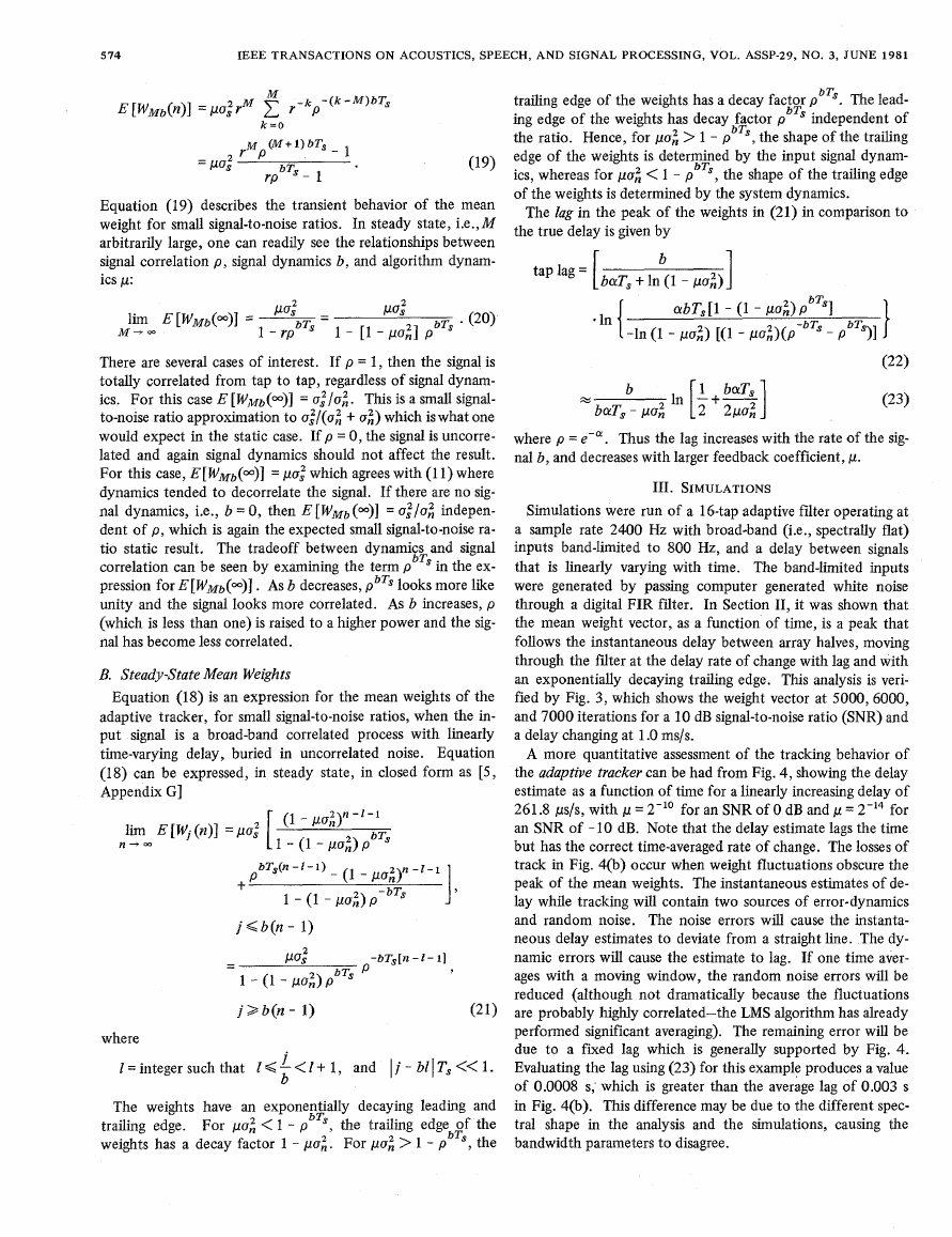
an exponentially decaying trailing edge. This analysis is veri-
fied by Fig. 3, which shows the weight vector at 5000,6000,
and 7000 iterations for a 10 dB signal-to-noise ratio (SNR) and
a delay changing at 1 .O ms/s.
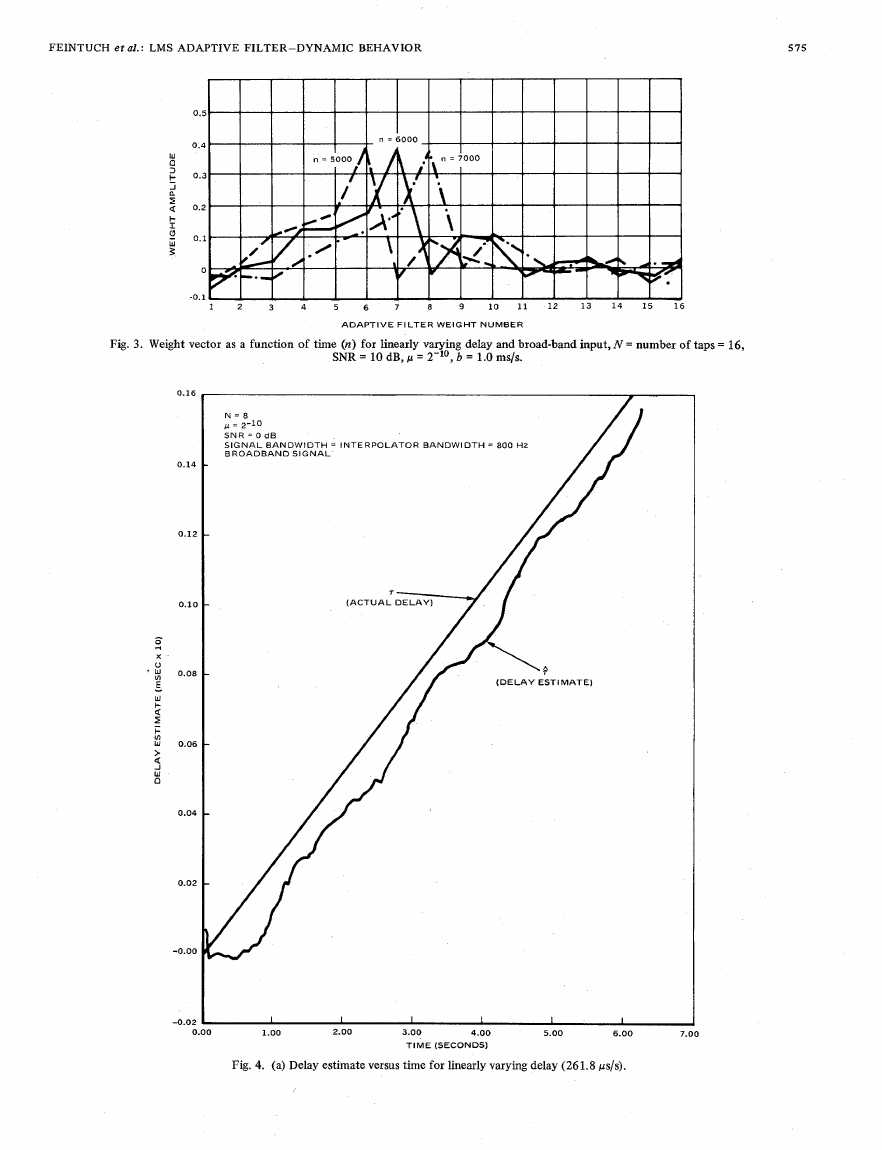
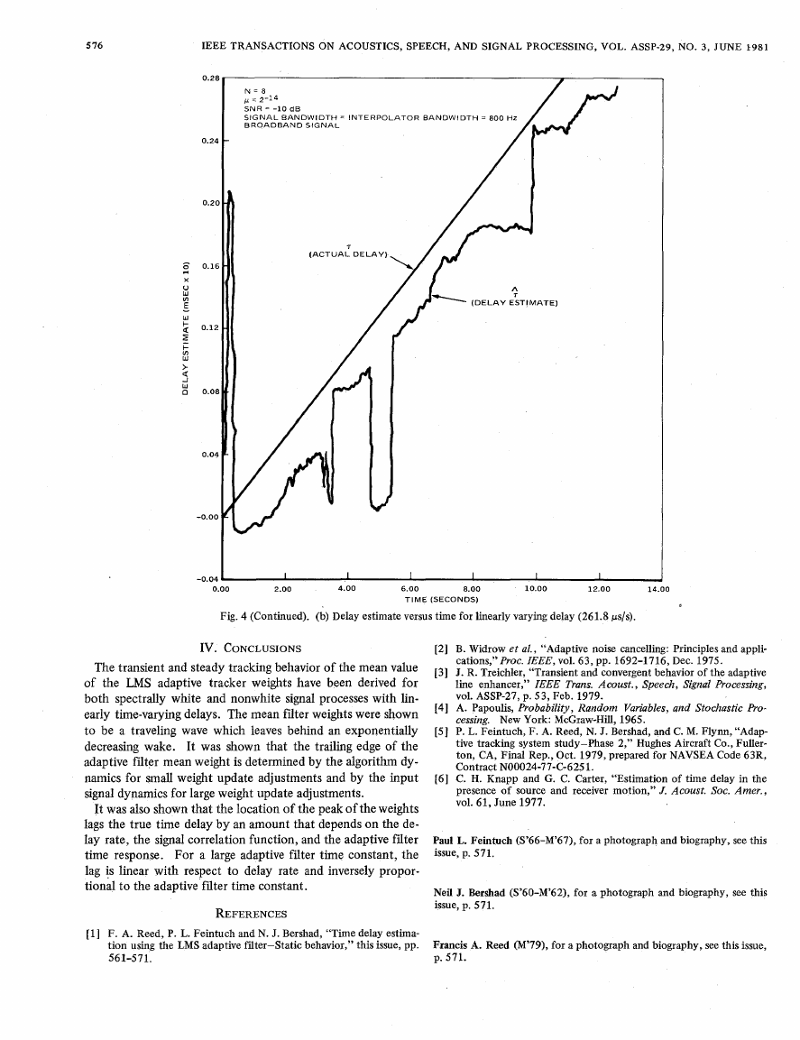
A more quantitative assessment of the tracking behavior of
the adaptive tracker can be had from Fig. 4, showing the delay
estimate as a function of time for a linearly increasing delay of
261.8 ps/s, with ,u = 2-l’
for an SNR of 0 dB and p = 2-14 for
an SNR of - 10 dB. Note that the delay estimate lags the time
but has the correct time-averaged rate of change. The losses of
track in Fig. 4(b) occur when weight fluctuations obscure the
peak of the mean weights. The instantaneous estimates of de-
lay while tracking will contain two sources of error-dynamics
and random noise. The noise errors will cause the instanta-
neous delay estimates to deviate from a straight line. The dy-
namic errors will cause the estimate to lag. If one time aver-
ages with a moving window, the random noise errors will be
reduced (although not dramatically because the fluctuations
are probably highly correlated-the LMS algorithm has already
performed significant averaging). The remaining error will be
due to a fixed lag which is generally supported by Fig. 4.
Evaluating the lag using (23) for this example produces a value
of 0.0008 s; which is greater than the average lag of 0.003 s
in Fig. 4(b). This difference may be due to the different spec-
tral shape in the
analysis and the simulations, causing the
bandwidth parameters to disagree.
�
FEINTUCH et al.: LMS ADAPTIVE FILTER-DYNAMIC BEHAVIOR
515
0
r(
X u
’
-
-
E
W 2
I
> 4
VI
W
n
0.16
0.14
0.12
0.10
0.08
0.06
0.04
0.02
-0.00
-0.02
Fig. 4. (a) Delay estimate versus time for linearly varying delay (261.8 ps/s).
T I M E (SECONDS)
�
576
IEEE TRANSACTIONS ON ACOUSTICS, SPEECH, AND SIGNAL PROCESSING, VOL. ASSP-29, NO. 3, JUNE 1981
N = 8
p = 2-14
SNR = -10 dB
SIGNAL BANDWIDTH = INTERPOLATOR BANDWIDTH = 800 Hz
BROADBAND SIGNAL
0.28
0.24 -
4
0.20
7
(ACTUAL DELAY)
8 0.16 7
X
I
u
VI
-
0.12
E -
w 2
s_
VI
> 4
0 0.08
0.04
1
I
\
-0.00
\
I
0.00
2.00
4.00
10.00
12.00
14.00
Fig. 4 (Continued). (6) Delay estimate versus time for linearly Varying delay (261.8 I.rS/s).
6.00
8.00
TIME (SECONDS)
IV. CONCLUSIONS
The transient and steady tracking behavior of the mean value
of the LMS adaptive tracker weights have been derived for
both spectrally white and nonwhite signal processes with lin-
early time-varying delays. The mean filter weights were shown
to be a traveling wave which leaves behind an exponentially
decreasing wake. It was shown that the trailing edge of the
adaptive filter mean weight is determined by the algorithm dy-
namics for small weight update adjustments and by the input
signal dynamics for large weight update adjustments.
It was also shown that the location of the peak of the weights
lags the true time delay by an amount that depends on the de-
lay rate, the signal correlation function, and the adaptive filter
time response. For a
lag is linear with respect to delay rate and inversely propor-
tional to the adaptive filter time constant.
large adaptive filter time constant, the
REFERENCES
[2] B. Widrow et al., “Adaptive noise cancelling: Principles and appli-
cations,” Proc. IEEE, vol. 63, pp. 1692-1716, Dec. 1975.
[3] J. R. Treichler, “Transient and convergent behavior of the adaptive
line enhancer,” IEEE Trans. Acoust., Speech, Signal Processing,
vol. ASSP-27, p. 53, Feb. 1979.
[4] A. Papoulis, Probability, Random Variables, and Stochastic Pro-
cessing. New York: McGraw-Hill, 1965.
[ 5 ] P. L. Feintuch, F. A. Reed, N. J. Bershad, and C. M. Flynn, “Adap-
tive tracking system study-Phase 2,” Hughes Aircraft Co., Fuller-
ton, CA, Final Rep., Oct. 1979, prepared for NAVSEA Code 63R,
Contract N00024-7746251.
[6] C. H. Knapp and G. C. Carter, “Estimation of time delay in the
presence of source and receiver motion,” J. Acoust. SOC. Amer.,
vol. 61, June 1977.
Neil J. Bershad (S’60-M’62), for a photograph and biography, see this
issue, p. 571.
[ l ] F. A. Reed, P. L. Feintuch and N. J. Bershad, “Time delay estima-
tion using the LMS adaptive Titer-Static behavior,” this issue, pp.
561-571.
Francis A. Reed (M’79), for a photograph and biography, see this issue,
p. 571.
�



 2023年江西萍乡中考道德与法治真题及答案.doc
 2012年重庆南川中考生物真题及答案.doc
 2013年江西师范大学地理学综合及文艺理论基础考研真题.doc
 2020年四川甘孜小升初语文真题及答案I卷.doc
 2020年注册岩土工程师专业基础考试真题及答案.doc
 2023-2024学年福建省厦门市九年级上学期数学月考试题及答案.doc
 2021-2022学年辽宁省沈阳市大东区九年级上学期语文期末试题及答案.doc
 2022-2023学年北京东城区初三第一学期物理期末试卷及答案.doc
 2018上半年江西教师资格初中地理学科知识与教学能力真题及答案.doc
 2012年河北国家公务员申论考试真题及答案-省级.doc
 2020-2021学年江苏省扬州市江都区邵樊片九年级上学期数学第一次质量检测试题及答案.doc
 2022下半年黑龙江教师资格证中学综合素质真题及答案.doc