Interactive graph cuts for optimal.pdf

发布时间：2022-06-08 发布人：admin 分类：说明书资料大小：0.28M 资料格式：pdf 举报版权申诉

第1页 / 共8页

第2页 / 共8页

第3页 / 共8页

第4页 / 共8页

第5页 / 共8页

第6页 / 共8页

第7页 / 共8页

第8页 / 共8页

文本预览

Proceedingsof“InternationConferenceonComputerVision”,Vancouver,Canada,July2001 vol.I,p.105 for Optimal Boundary & Region Segmentation of Objects in N-D Images Interactive Graph Cuts Yuri Y. Boykov Marie-Pierre Jolly Siemens Corporate Research 755 College Road East, Princeton, NJ 08540, USA yuri@csd.uwo.ca Abstract In this paper we describe a new technique for general purpose interactive segmentation of N-dimensional images. The user marks certain pixels as “object” or “background” to provide hard constraints for segmentation. Additional soft constraints incorporate both boundary and region in- formation. Graph cuts are used to ﬁnd the globally optimal segmentation of the N-dimensional image. The obtained so- lution gives the best balance of boundary and region prop- erties among all segmentations satisfying the constraints. The topology of our segmentation is unrestricted and both “object” and “background” segments may consist of sev- eral isolated parts. Some experimental results are presented in the context of photo/video editing and medical image seg- mentation. We also demonstrate an interesting Gestalt ex- ample. A fast implementation of our segmentation method is possible via a new max-ﬂow algorithm in [2]. 1. Introduction Interactive segmentation is becoming more and more popular to alleviate the problems inherent to fully automatic segmentation which seems to never be perfect. Our goal is a general purpose interactive segmentation technique that divides an image into two segments: “object” and “back- ground”. A user imposes certain hard constraints for seg- mentation by indicating certain pixels (seeds) that abso- lutely have to be part of the object and certain pixels that have to be part of the background. Intuitively, these hard constraints provide clues on what the user intends to seg- ment. The rest of the image is segmented automatically by computing a global optimum among all segmentations sat- isfying the hard constraints. The cost function is deﬁned in terms of boundary and region properties of the segments. These properties can be viewed as soft constraints for seg- mentation. A globally optimal segmentation can be very efﬁciently recomputed when the user adds or removes any hard constraints (seeds). This allows the user to get any desired segmentation results quickly via very intuitive in- teractions. Our method applies to N-D images (volumes). One of the main advantages of our interactive segmen- tation method is that it provides a globally optimal solution for an N-dimensional segmentation when the cost function is clearly deﬁned. Some earlier techniques (snakes [14, 4], deformable templates [21], shortest path [15], ratio regions [5], and other [13]) can do that only in 2D applications when a segmentation boundary is a 1D curve. Many techniques either don’t have a clear cost function at all (region growing, split and merge, see Chapter 10 in [11]) or compute only an approximate solution (e.g. a local minimum) that can be arbitrarily far from the global optimum (region competition [22], level set methods [16], normalized cuts [18]). Global properties of such segmentations may be difﬁcult to analyze or predict. Imperfections in the result might come from de- ﬁciencies at the minimization stage. In contrast, imperfec- tions of a globally optimal solution are directly related to the deﬁnition of the cost function. Thus, the segmentation can be controlled more reliably. It is also important that the cost function that we use as a soft constraint for segmentation is general enough to include both region and boundary properties of segments. In fact, our cost function is similar to one in [9] obtained in a context of MAP-MRF estimation. Consider an arbi- trary set of data elements P and some neighborhood sys- tem represented by a set N of all unordered1 pairs {p, q} of neighboring elements in P. For example, P can con- tain pixels (or voxels) in a 2D (or 3D) grid and N can 1For simplicity, we present the case of unordered pairs of neighbors {p, q}. If pairs of neighbors are ordered then we have two distinct pairs (p, q) and (q, p). This would allow different (directed) discontinuity penalties for two cases when p ∈ “object”, q ∈ “background” and when p ∈ “background”, q ∈ “object”. To set such directed costs one should have prior information on properties of the boundary from object to back- ground. Algorithmically, generalization from unordered to ordered neigh- bors means switching from undirected (presented here) to directed graphs.

Proceedingsof“InternationConferenceonComputerVision”,Vancouver,Canada,July2001 vol.I,p.106 contain all unordered pairs of neighboring pixels (voxels) under a standard 8- (or 26-) neighborhood system. Let A = (A1, . . . , Ap, . . . , A|P|) be a binary vector whose components Ap specify assignments to pixels p in P. Each Ap can be either “obj” or “bkg” (abbreviations of “object” and “background”). Vector A deﬁnes a segmentation. Then, the soft constraints that we impose on boundary and region properties of A are described by the cost function E(A): where and E(A) = λ · R(A) + B(A) Rp(Ap) R(A) = Xp∈P B(A) = X{p,q}∈N B{p,q} · δ(Ap, Aq) δ(Ap, Aq) = 1 if Ap 6= Aq otherwise. 0 (1) (2) (3) The coefﬁcient λ ≥ 0 in (1) speciﬁes a relative impor- tance of the region properties term R(A) versus the bound- ary properties term B(A). The regional term R(A) as- sumes that the the individual penalties for assigning pixel p to “object” and “background”, correspondingly Rp(“obj”) and Rp(“bkg”), are given. For example, Rp(·) may reﬂect on how the intensity of pixel p ﬁts into a known intensity model (e.g. histogram) of the object and background. The term B(A) comprises the “boundary” properties of segmentation A. Coefﬁcient B{p,q} ≥ 0 should be inter- preted as a penalty for a discontinuity between p and q. Nor- mally, B{p,q} is large when pixels p and q are similar (e.g. in their intensity) and B{p,q} is close to zero when the two are very different. The penalty B{p,q} can also decrease as a function of distance between p and q. Costs B{p,q} may be based on local intensity gradient, Laplacian zero-crossing, gradient direction, and other criteria (e.g. [15]). The algorithm in [9] computes a globally optimal binary segmentation minimizing the energy similar to (1) when no hard constraints are placed. In contrast, our goal is to com- pute the global minimum of (1) among all segmentations that satisfy additional hard constraints imposed by a user. There are different types of hard constraints that were proposed in the past for interactive segmentation methods. For example, for intelligent scissors [15] and live wire [6], the user has to indicate certain pixels where the segmenta- tion boundary should pass. The segmentation boundary is then computed as the “shortest path” between the marked pixels according to some energy function based on image gradient. One difﬁculty with such hard constraints is that the user inputs have to be very accurately positioned at the desired boundary. Moreover, this approach can not be easily generalized to 3D data. We consider hard constraints that indicate segmentation regions rather than the boundary. We assume that some pix- els were marked as internal and some as external for the given object of interest. The subsets of marked pixels will be referred to as “object” and “background” seeds. The seg- mentation boundary can be anywhere but it has to separate the object seeds from the background seeds. Note that the seeds can be loosely positioned inside the object and back- ground regions. Our segmentation technique is quite stable and normally produces the same results regardless of par- ticular seed positioning within the same image object. Obviously, the hard constraints by themself are not enough to obtain a good segmentation. A segmentation method decides how to segment unmarked pixels. [10] and [17] use the same type of hard constraints as us but they do not employ a clear cost function and segment unmarked pixels based on variations of “region growing”. Since the properties of segmentation boundary are not optimized, the results are prone to “leaking” where the boundary between objects is blurry. In contrast, we combine the hard con- straints as above with energy (1) that incorporates region and boundary properties of segments. In this paper we show how to generalize the algorithm in [9] to combine soft constraints encoded in (1) with user deﬁned hard constraints. We also show how the optimal segmentations can be efﬁciently recomputed if the hard con- straints are added or changed. Note that initial segmentation may not be perfect. After reviewing it, the user can specify additional object and background seeds depending on the observed results. To incorporate these new seeds the algo- rithm can efﬁciently adjust the current segmentation with- out recomputing the whole solution from scratch. Our technique is based on powerful graph cut algorithms from combinatorial optimization [7, 8]. Our implementa- tion uses a new version of “max-ﬂow” algorithm reported in [2]. In the next section we explain the terminology for graph cuts and provide some background information on previous computer vision techniques relying on graph cuts. The details of our segmentation method and its correctness are shown in Section 3. Section 4 provides a number of examples where we apply our technique to photo/video- editing and to segmentation of medical images/volumes. We demonstrate that with a few simple and intuitive ma- nipulations a user can always segment an object of interest as precisely as (s)he wants. Note that some additional ex- perimental results can be found in our preliminary work [1] which can be seen as a restricted case where only bound- ary term is present in energy (1). Information on possible extensions and future work is given in Section 5.

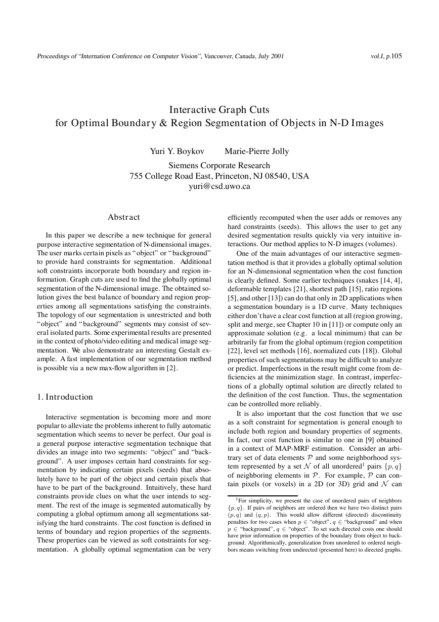
Proceedingsof“InternationConferenceonComputerVision”,Vancouver,Canada,July2001 vol.I,p.107 (a) Image with seeds. (d) Segmentation results. ⇓ ⇑ ⇒ (b) Graph. (c) Cut. Figure 1. A simple 2D segmentation example for a 3 × 3 image. The seeds are O = {v} and B = {p}. The cost of each edge is reﬂected by the edge’s thickness. The regional term (2) and hard constraints (4,5) deﬁne the costs of t-links. The boundary term (3) deﬁnes the costs of n-links. Inexpensive edges are at- tractive choices for the minimum cost cut. 2. Graph Cuts and Computer Vision First, we describe the basic terminology that pertains to graph cuts in the context of our segmentation method. An undirected graph G = hV, Ei is deﬁned as a set of nodes (vertices V) and a set of undirected edges (E) that connect these nodes. An example of a graph that we use in this paper is shown in Figure 1(b). Each edge e ∈ E in the graph is assigned a nonnegative weight (cost) we. There are also two special nodes called terminals. A cut is a subset of edges C ⊂ E such that the terminals become separated on the induced graph G(C) = hV, E\Ci. It is normal in combinatorial optimization to deﬁne the cost of a cut as the sum of the costs of the edges that it severs |C| = Xe∈C we. the nodes in the graph. As illustrated in Figure 1 (c-d), this partitioning corresponds to a segmentation of an underlying image or volume. A minimum cost cut generates a segmen- tation that is optimal in terms of properties that are built into the edge weights. Our technique is based on a well-known combinatorial optimization fact that a globally minimum cut of a graph with two terminals can be computed efﬁciently in low-order polynomial time [7, 8, 2]. In Section 3 we show how to set a two terminal graph so that the minimum cut would give a segmentation that minimizes (1) among all segmentations satisfying the given hard constraints. It should be noted that graph cuts were used for image segmentation before. In [20] the image is optimally divided into K parts to minimize the maximum cut between the seg- ments. In this formulation, however, the segmentation is strongly biased to very small segments. Shi and Malik [18] try to solve this problem by normalizing the cost of a cut. The resulting optimization problem is NP-hard and they use an approximation technique. In [9, 3, 12, 19] graph cuts are applied to minimize certain energy functions used in im- age restoration, stereo, 3D object reconstruction, and other problems in computer vision. A fast implementation of theoretically polynomial graph cut algorithms can be an issue. The most straight-forward implementations of the standard graph cut algorithms, e.g. max-ﬂow [7] or push-relabel [8], can be slow. The experi- ments in [2] compare several well-known “tuned” versions of these standard algorithms in the context of graph based methods in vision. The same paper also describes a new ver- sion of the max-ﬂow algorithm that (on typical in vision ex- amples) signiﬁcantly outperformed the standard techniques. Our implementation of the interactive segmentation method of this paper uses the new graph cut algorithm from [2]. 3. Segmentation Technique In this section we provide algorithmic details about our segmentation technique. Assume that O and B denote the subsets of pixels marked as “object” and “background” seeds. Naturally, the subsets O ⊂ P and B ⊂ P are such that O ∩ B = ∅. Remember that our goal is to compute the global minimum of (1) among all segmentations A satisfy- ing hard constraints ∀p ∈ O, ∀p ∈ B, Ap = “obj” Ap = “bkg”. (4) (5) Graph cut formalism is well suited for segmentation of images. In fact, it is completely appropriate for N- dimensional volumes. The nodes of the graph can represent pixels (or voxels) and the edges can represent any neigh- borhood relationship between the pixels. A cut partitions The general work ﬂow is shown in Figure 1. Given an image (Figure 1(a)) we create a graph with two terminals (Figure 1(b)). The edge weights reﬂect the parameters in the regional (2) and the boundary (3) terms of the cost func- tion, as well as the known positions of seeds in the image.

Proceedingsof“InternationConferenceonComputerVision”,Vancouver,Canada,July2001 vol.I,p.108 The next step is to compute the globally optimal minimum cut (Figure 1(c)) separating two terminals. This cut gives a segmentation (Figure 1(d)) of the original image. In the simplistic example of Figure 1 the image is divided into ex- actly one “object” and one “background” regions. In gen- eral, our segmentation method generates binary segmenta- tion with arbitrary topological properties. Examples in Sec- tion 4 illustrate that object and background segments may consist of several isolated connected blobs in the image. Below we describe the details of the graph and prove that the obtained segmentation is optimal. To segment a given image we create a graph G = hV, Ei with nodes cor- responding to pixels p ∈ P of the image. There are two additional nodes: an “object” terminal (a source S) and a “background” terminal (a sink T ). Therefore, V = P ∪ {S, T }. The set of edges E consists of two types of undirected edges: n-links (neighborhood links) and t-links (terminal links). Each pixel p has two t-links {p, S} and {p, T } connecting it to each terminal. Each pair of neighboring pixels {p, q} in N is connected by an n-link. Without introducing any ambiguity, an n-link connecting a pair of neighbors p and q will be denoted by {p, q}. Therefore, E = N [p∈P {{p, S}, {p, T }}. The following table gives weights of edges in E edge weight (cost) for {p, q} B{p,q} {p, q} ∈ N (see Section 2) assuming that the edge weights speciﬁed in the table above are non-negative2. Below we state exactly how the minimum cut ˆC deﬁnes a segmentation ˆA and prove this segmentation is optimal. We need one technical lemma. Assume that F denotes a set of all feasible cuts C on graph G such that • C severs exactly one t-link at each p • {p, q} ∈ C iff p, q are t-linked to different terminals • if p ∈ O then {p, T } ∈ C • if p ∈ B then {p, S} ∈ C. Lemma 1 The minimum cut on G is feasible, i.e. ˆC ∈ F. ˆC severs et least one t-link at each pixel since it PROOF: is a cut that separates the terminals. On the other hand, it can not sever both t-links. In such a case it would not be minimal since one of the t-links could be returned. Simi- larly, a minimum cut should sever an n-link {p, q} if p and q are connected to the opposite terminals just because any cut must separate the terminals. If p and q are connected to the same terminal then ˆC should not sever unnecessary n-link {p, q} due to its minimality. The last two properties are true for ˆC because the constant K is larger than the sum of all n-links costs for any given pixel p. For example, if p ∈ O and ˆC severs {p, S} (costs K) then we would con- struct a smaller cost cut by restoring {p, S} and severing all n-links from p (costs less then K) as well as the opposite t-link {p, T } (zero cost). λ · Rp(“bkg”) p ∈ P, p 6∈ O ∪ B For any feasible cut C ∈ F we can deﬁne a unique cor- responding segmentation A(C) such that {p, S} {p, T } K 0 p ∈ O p ∈ B λ · Rp(“obj”) p ∈ P, p 6∈ O ∪ B 0 K p ∈ O p ∈ B where K = 1 + max p∈P Xq: {p,q}∈N B{p,q}. Ap(C) = “obj”, “bkg”, if {p, T } ∈ C if {p, S} ∈ C. (6) The deﬁnition above is coherent since any feasible cut sev- ers exactly one of the two t-links at each pixel p. The lemma showed that a minimum cut ˆC is feasible. Thus, we can de- ﬁne a corresponding segmentation ˆA = A( ˆC). The next theorem completes the description of our algorithm. Theorem 1 The segmentation ˆA = A( ˆC) deﬁned by the minimum cut ˆC as in (6) minimizes (1) among all segmen- tations satisfying constraints (4,5). The graph G is now completely deﬁned. We draw the segmentation boundary between the object and the back- ground by ﬁnding the minimum cost cut on the graph G. The minimum cost cut ˆC on G can be computed exactly in polynomial time via algorithms for two terminal graph cuts 2In fact, our technique does require that the penalties B{p,q} be non- negative. The restriction that Rp(·) should be non-negative is easy to avoid. For any pixel p we can always add a large enough positive con- stant to both Rp(“obj”) and Rp(“bkg”) to make sure that they become non-negative. This operation can not change the minimum A of E(A) in (1) since it is equivalent to adding a constant to the whole energy function.

Proceedingsof“InternationConferenceonComputerVision”,Vancouver,Canada,July2001 vol.I,p.109 PROOF: Using the table of edge weights, deﬁnition of fea- sible cuts F, and equation (6) one can show that a cost of any C ∈ F is |C| = Xp6∈O∪B X{p,q}∈N λ · Rp(Ap(C)) + B{p,q} · δ(Ap(C), Aq(C)) = E(A(C)) − Xp∈O λRp(“obj”) − Xp∈B λRp(“bkg”). Therefore, |C| = E(A(C)) − const(C). Note that for any C ∈ F assignment A(C) satisﬁes constraints (4,5). In fact, equation (6) gives a one-to-one correspondence between the set of all feasible cuts in F and the set H of all assignments A that satisfy hard constraints (4,5). Then, E( ˆA) = | ˆC| + const = min C∈F |C| + const = t-link initial cost add new cost {p, S} λRp(“bkg”) K + λRp(“obj”) K + cp {p, T } λRp(“obj”) λRp(“bkg”) cp These new costs are consistent with the edge weight table for pixels in O since the extra constant cp at both t-links of a pixel does not change the optimal cut4. Then, a maximum ﬂow (minimum cut) on a new graph can be efﬁciently ob- tained starting from the previous ﬂow without recomputing the whole solution from scratch. Note that the same trick can be done to adjust the seg- mentation when a new “background” seed is added or when a seed is deleted. One has to ﬁgure the right amounts that have to be added to the costs of two t-links at the corre- sponding pixel. The new costs should be consistent with the edge weight table plus or minus the same constant. = min C∈F E(A(C)) = min A∈H E(A) 4. Examples and the theorem is proved. To conclude this section we would like to show that our algorithm can efﬁciently adjust the segmentation to incor- porate any additional seeds that the user might interactively add. To be speciﬁc, assume that a max-ﬂow algorithm is used to determine the minimum cut on G. The max-ﬂow algorithm gradually increases the ﬂow sent from the source S to the sink T along the edges in G given their capacities (weights). Upon termination the maximum ﬂow saturates3 the graph. The saturated edges correspond to the minimum cost cut on G giving us an optimal segmentation. Assume now that an optimal segmentation is already computed for some initial set of seeds. A user adds a new “object” seed to pixel p that was not previously assigned any seed. We need to change the costs for two t-links at p t-link initial cost new cost {p, S} λRp(“bkg”) {p, T } λRp(“obj”) K 0 and then compute the maximum ﬂow (minimum cut) on the new graph. In fact, we can start from the ﬂow found at the end of initial computation. The only problem is that re- assignment of edge weights as above reduces capacities of some edges. If there is a ﬂow through such an edge then we may break the ﬂow consistency. Increasing an edge ca- pacity, on the other hand, is never a problem. Then, we can solve the problem as follows. To accommodate the new “object” seed at pixel p we increase the t-links weights according to the table 3See [7] or [2] for details. We demonstrate our general-purpose segmentation method in several examples including photo/video editing and medical data processing. We show original data and segments generated by our technique for a given set of seeds. Our actual interface allows a user to enter seeds via mouse operated brush of red (for object) or blue (for back- ground) color. Due to limitations of this B&W publication we show seeds as strokes of white (object) or black (back- ground) brush. In addition, these strokes are marked by the letters “O” and “B”. For the purpose of clarity, we employ different methods for the presentation of segmentation re- sults in our examples below. Our current implementation actually makes a double use of the seeds entered by a user. First of all, they provide the hard constraints for the segmentation process as dis- cussed in Section 3. In addition, we use intensities of pix- els (voxels) marked as seeds to get histograms for “ob- ject” and “background” intensity distributions: Pr(I|O) and Pr(I|B)5. Then, we use these histograms to set the regional penalties Rp(·) as negative log-likelihoods: Rp(“obj”) = − ln Pr(Ip|O) Rp(“bkg”) = − ln Pr(Ip|B). Such penalties are motivated by the underlying MAP-MRF formulation [9, 3]. To set the boundary penalties we use an ad-hoc function B{p,q} ∝ exp− (Ip − Iq)2 2σ2 · 1 dist(p, q) . 4Note that the minimum cut severs exactly one of two t-links at pixel p. 5Alternatively, the histograms can be learned from historic data.

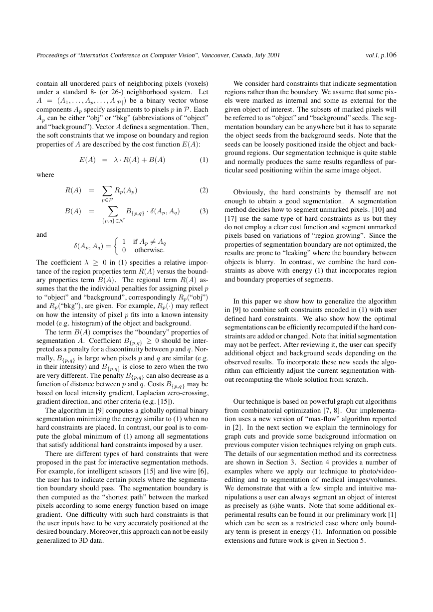
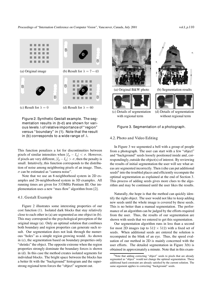
Proceedingsof“InternationConferenceonComputerVision”,Vancouver,Canada,July2001 vol.I,p.110 (a) Original image (b) Result for λ = 7—43 (c) Result for λ = 0 (d) Result for λ = 60 Figure 2. Synthetic Gestalt example. The seg- mentation results in (b-d) are shown for vari- ous levels λ of relative importance of “region” versus “boundary” in (1). Note that the result in (b) corresponds to a wide range of λ. This function penalizes a lot for discontinuities between pixels of similar intensities when |Ip − Iq| < σ. However, if pixels are very different, |Ip − Iq| > σ, then the penalty is small. Intuitively, this function corresponds to the distribu- tion of noise among neighboring pixels of an image. Thus, σ can be estimated as “camera noise”. Note that we use an 8-neighborhood system in 2D ex- amples and 26-neighborhood system in 3D examples. All running times are given for 333MHz Pentium III. Our im- plementation uses a new “max-ﬂow” algorithm from [2]. 4.1. Gestalt Example Figure 2 illustrates some interesting properties of our cost function (1). Isolated dark blocks that stay relatively close to each other in (a) are segmented as one object in (b). This may correspond to the psychological perception of the original image (a). Only an optimal solution that combines both boundary and region properties can generate such re- sult. Our segmentation does not leak through the numer- ous “holes” as a simple region growing would. As shown in (c), the segmentation based on boundary properties only “shrinks” the object. The opposite extreme when the region properties strongly dominate the boundary forces is shown in (d). In this case the method creates isolated segments for individual blocks. The bright space between the blocks has a better ﬁt with the “background” histogram and the super- strong regional term forces the “object” segment out. 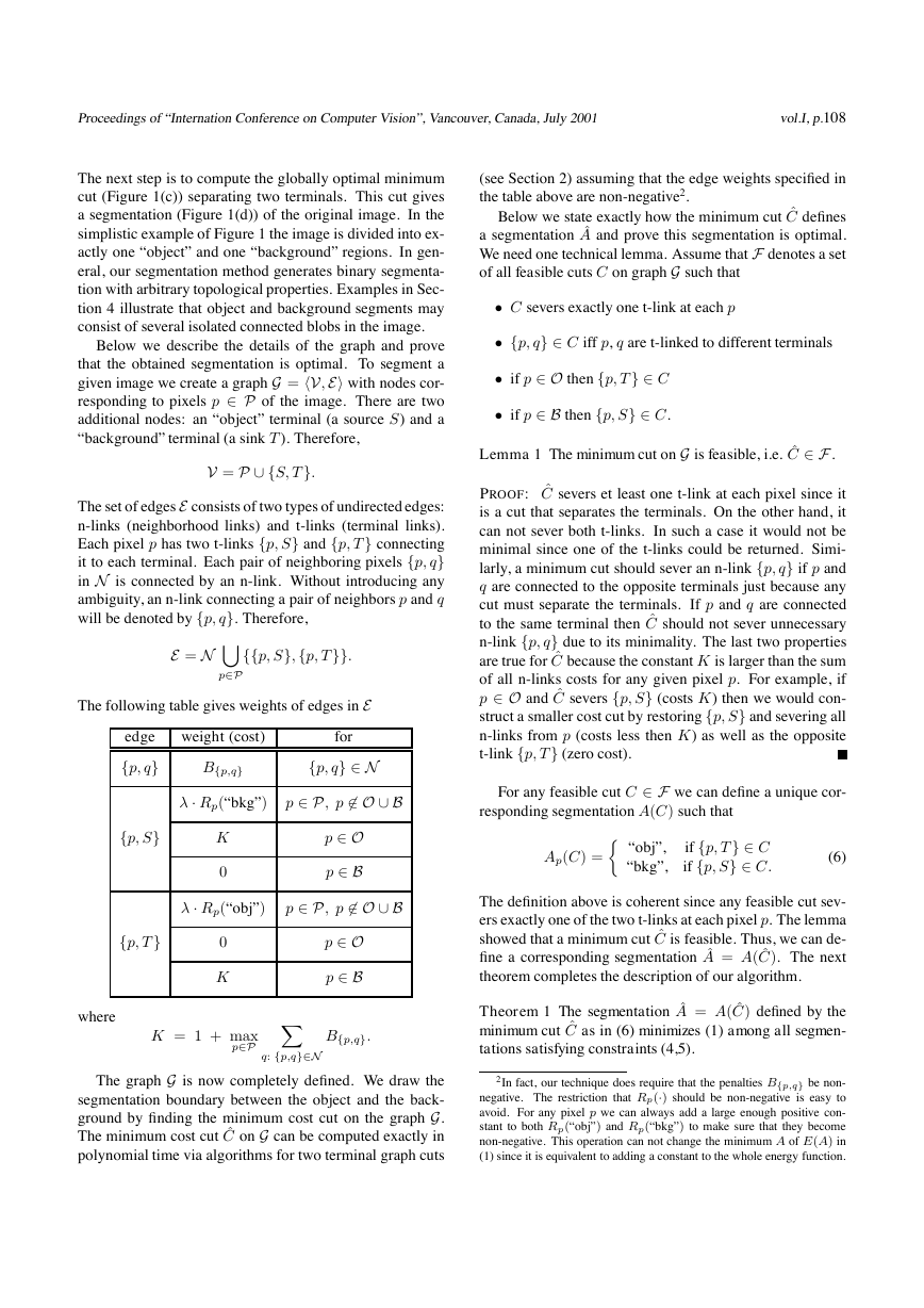(a) Original B&W photo (b) Segmentation results (c) Details of segmentation (d) Details of segmentation with regional term without regional term Figure 3. Segmentation of a photograph. 4.2. 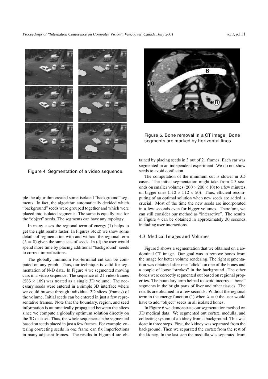Photo and Video Editing In Figure 3 we segmented a bell with a group of people from a photograph. The user can start with a few “object” and “background” seeds loosely positioned inside and, cor- respondingly, outside the object(s) of interest. By reviewing the results of initial segmentation the user will see what ar- eas are segmented incorrectly. Then (s)he can put additional seeds6 into the troubled places and efﬁciently recompute the optimal segmentation as explained at the end of Section 3. This process of adding seeds gives more clues to the algo- rithm and may be continued until the user likes the results. Naturally, the hope is that the method can quickly iden- tify the right object. The user would not like to keep adding new seeds until the whole image is covered by these seeds. This is no better than a manual segmentation. The perfor- mance of an algorithm can be judged by the efforts required from the user. Thus, the results of our segmentation are shown with seeds that we entered to get this segmentation. Our segmentation algorithm runs in less than a second for most 2D images (up to 512 × 512) with a ﬁxed set of seeds. When additional seeds are entered the solution is recomputed in the blink of an eye. Thus, the speed eval- uation of our method in 2D is mainly concerned with the user efforts. The detailed segmentation in Figure 3(b) is obtained in approximately a minute. Note that in this exam- 6Note that adding correcting “object” seeds to pixels that are already segmented as “object” would not change the optimal segmentation. These additional hard constraint are already satisﬁed by the current solution. The same argument applies to correcting “background” seeds.

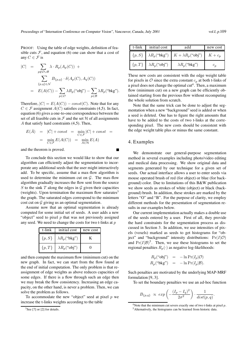
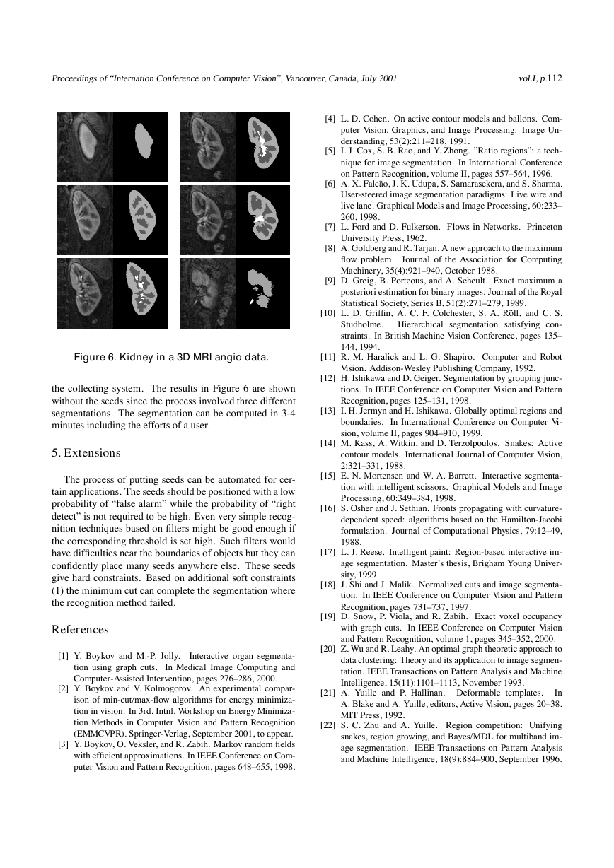
Proceedingsof“InternationConferenceonComputerVision”,Vancouver,Canada,July2001 vol.I,p.111 Figure 4. Segmentation of a video sequence. ple the algorithm created some isolated “background” seg- ments. In fact, the algorithm automatically decided which “background” seeds were grouped together and which were placed into isolated segments. The same is equally true for the “object” seeds. The segments can have any topology. In many cases the regional term of energy (1) helps to get the right results faster. In Figures 3(c,d) we show some details of segmentation with and without the regional term (λ = 0) given the same sets of seeds. In (d) the user would spend more time by placing additional “background” seeds to correct imperfections. The globally minimum two-terminal cut can be com- puted on any graph. Thus, our technique is valid for seg- mentation of N-D data. In Figure 4 we segmented moving cars in a video sequence. The sequence of 21 video frames (255 × 189) was treated as a single 3D volume. The nec- essary seeds were entered in a simple 3D interface where we could browse through individual 2D slices (frames) of the volume. Initial seeds can be entered in just a few repre- sentative frames. Note that the boundary, region, and seed information is automatically propagated between the slices since we compute a globally optimum solution directly on the 3D data set. Thus, the whole sequence can be segmented based on seeds placed in just a few frames. For example, en- tering correcting seeds in one frame can ﬁx imperfections in many adjacent frames. The results in Figure 4 are ob- Figure 5. Bone removal in a CT image. Bone segments are marked by horizontal lines. tained by placing seeds in 3 out of 21 frames. Each car was segmented in an independent experiment. We do not show seeds to avoid confusion. The computation of the minimum cut is slower in 3D cases. The initial segmentation might take from 2-3 sec- onds on smaller volumes (200 × 200 × 10) to a few minutes on bigger ones (512 × 512 × 50). Thus, efﬁcient recom- puting of an optimal solution when new seeds are added is crucial. Most of the time the new seeds are incorporated in a few seconds even for bigger volumes. Therefore, we can still consider our method as “interactive”. The results in Figure 4 can be obtained in approximately 30 seconds including user interactions. 4.3. Medical Images and Volumes Figure 5 shows a segmentation that we obtained on a ab- dominal CT image. Our goal was to remove bones from the image for better volume rendering. The right segmenta- tion was obtained after one “click” on one of the bones and a couple of loose “strokes” in the background. The other bones were correctly segmented out based on regional prop- erties. The boundary term helped to avoid incorrect “bone” segments in the bright parts of liver and other tissues. The results are obtained in a few seconds. Without the regional term in the energy function (1) when λ = 0 the user would have to add “object” seeds in all isolated bones. In Figure 6 we demonstrate our segmentation method on 3D medical data. We segmented out cortex, medulla, and collecting system of a kidney from a background. This was done in three steps. First, the kidney was separated from the background. Then we separated the cortex from the rest of the kidney. In the last step the medulla was separated from

Proceedingsof“InternationConferenceonComputerVision”,Vancouver,Canada,July2001 vol.I,p.112 [4] L. D. Cohen. On active contour models and ballons. Com- puter Vision, Graphics, and Image Processing: Image Un- derstanding, 53(2):211–218, 1991. [5] I. J. Cox, S. B. Rao, and Y. Zhong. ”Ratio regions”: a tech- nique for image segmentation. In International Conference on Pattern Recognition, volume II, pages 557–564, 1996. [6] A. X. Falc˜ao, J. K. Udupa, S. Samarasekera, and S. Sharma. User-steered image segmentation paradigms: Live wire and live lane. Graphical Models and Image Processing, 60:233– 260, 1998. [7] L. Ford and D. Fulkerson. Flows in Networks. Princeton University Press, 1962. [8] A. Goldberg and R. Tarjan. A new approach to the maximum ﬂow problem. Journal of the Association for Computing Machinery, 35(4):921–940, October 1988. [9] D. Greig, B. Porteous, and A. Seheult. Exact maximum a posteriori estimation for binary images. Journal of the Royal Statistical Society, Series B, 51(2):271–279, 1989. [10] L. D. Grifﬁn, A. C. F. Colchester, S. A. R¨oll, and C. S. Studholme. Hierarchical segmentation satisfying con- straints. In British Machine Vision Conference, pages 135– 144, 1994. [11] R. M. Haralick and L. G. Shapiro. Computer and Robot Vision. Addison-Wesley Publishing Company, 1992. [12] H. Ishikawa and D. Geiger. Segmentation by grouping junc- tions. In IEEE Conference on Computer Vision and Pattern Recognition, pages 125–131, 1998. [13] I. H. Jermyn and H. Ishikawa. Globally optimal regions and In International Conference on Computer Vi- boundaries. sion, volume II, pages 904–910, 1999. [14] M. Kass, A. Witkin, and D. Terzolpoulos. Snakes: Active contour models. International Journal of Computer Vision, 2:321–331, 1988. [15] E. N. Mortensen and W. A. Barrett. Interactive segmenta- tion with intelligent scissors. Graphical Models and Image Processing, 60:349–384, 1998. [16] S. Osher and J. Sethian. Fronts propagating with curvature- dependent speed: algorithms based on the Hamilton-Jacobi formulation. Journal of Computational Physics, 79:12–49, 1988. [17] L. J. Reese. Intelligent paint: Region-based interactive im- age segmentation. Master’s thesis, Brigham Young Univer- sity, 1999. [18] J. Shi and J. Malik. Normalized cuts and image segmenta- tion. In IEEE Conference on Computer Vision and Pattern Recognition, pages 731–737, 1997. [19] D. Snow, P. Viola, and R. Zabih. Exact voxel occupancy with graph cuts. In IEEE Conference on Computer Vision and Pattern Recognition, volume 1, pages 345–352, 2000. [20] Z. Wu and R. Leahy. An optimal graph theoretic approach to data clustering: Theory and its application to image segmen- tation. IEEE Transactions on Pattern Analysis and Machine Intelligence, 15(11):1101–1113, November 1993. [21] A. Yuille and P. Hallinan. Deformable templates. In A. Blake and A. Yuille, editors, Active Vision, pages 20–38. MIT Press, 1992. [22] S. C. Zhu and A. Yuille. Region competition: Unifying snakes, region growing, and Bayes/MDL for multiband im- age segmentation. IEEE Transactions on Pattern Analysis and Machine Intelligence, 18(9):884–900, September 1996. Figure 6. Kidney in a 3D MRI angio data. the collecting system. The results in Figure 6 are shown without the seeds since the process involved three different segmentations. The segmentation can be computed in 3-4 minutes including the efforts of a user. 5. Extensions The process of putting seeds can be automated for cer- tain applications. The seeds should be positioned with a low probability of “false alarm” while the probability of “right detect” is not required to be high. Even very simple recog- nition techniques based on ﬁlters might be good enough if the corresponding threshold is set high. Such ﬁlters would have difﬁculties near the boundaries of objects but they can conﬁdently place many seeds anywhere else. These seeds give hard constraints. Based on additional soft constraints (1) the minimum cut can complete the segmentation where the recognition method failed. References [1] Y. Boykov and M.-P. Jolly. tion using graph cuts. Computer-Assisted Intervention, pages 276–286, 2000. Interactive organ segmenta- In Medical Image Computing and [2] Y. Boykov and V. Kolmogorov. An experimental compar- ison of min-cut/max-ﬂow algorithms for energy minimiza- tion in vision. In 3rd. Intnl. Workshop on Energy Minimiza- tion Methods in Computer Vision and Pattern Recognition (EMMCVPR). Springer-Verlag, September 2001, to appear. [3] Y. Boykov, O. Veksler, and R. Zabih. Markov random ﬁelds with efﬁcient approximations. In IEEE Conference on Com- puter Vision and Pattern Recognition, pages 648–655, 1998.

分享到：

赞收藏

资料库

Interactive graph cuts for optimal.pdf

相关推荐

课程资源

热门标签

最新资料