Mathematical Biosciences 180 (2002) 29–48
www.elsevier.com/locate/mbs
Reproduction numbers and sub-threshold endemic
equilibria for compartmental models of disease transmission
P. van den Driessche a,1, James Watmough b,*,2
a Department of Mathematics and Statistics, University of Victoria, Victoria, BC, Canada V8W 3P4
b Department of Mathematics and Statistics, University of New Brunswick, Fredericton, NB, Canada E3B 5A3
Received 26 April 2001; received in revised form 27 June 2001; accepted 27 June 2001
Dedicated to the memory of John Jacquez
Abstract
A precise definition of the basic reproduction number, R0, is presented for a general compartmental
disease transmission model based on a system of ordinary differential equations. It is shown that, if R0 < 1,
then the disease free equilibrium is locally asymptotically stable; whereas if R0 > 1, then it is unstable.
Thus, R0 is a threshold parameter for the model. An analysis of the local centre manifold yields a simple
criterion for the existence and stability of super- and sub-threshold endemic equilibria for R0 near one. This
criterion, together with the definition of R0, is illustrated by treatment, multigroup, staged progression,
multistrain and vector–host models and can be applied to more complex models. The results are significant
for disease control.
Ó 2002 Elsevier Science Inc. All rights reserved.
Keywords: Basic reproduction number; Sub-threshold equilibrium; Disease transmission model; Disease control
1. Introduction
One of the most important concerns about any infectious disease is its ability to invade a
population. Many epidemiological models have a disease free equilibrium (DFE) at which the
* Corresponding author. Tel.: +1-506 458 7323; fax: +1-506 453 4705.
E-mail addresses: pvdd@math.uvic.ca (P. van den Driessche), watmough@unb.ca (J. Watmough).
URL: http://www.math.unb.ca/�watmough.
1 Research supported in part by an NSERC Research Grant, the University of Victoria Committee on faculty
research and travel and MITACS.
2 Research supported by an NSERC Postdoctoral Fellowship tenured at the University of Victoria.
0025-5564/02/$ - see front matter Ó 2002 Elsevier Science Inc. All rights reserved.
PII: S 0 0 2 5 - 5 5 6 4 ( 0 2 ) 0 0 1 0 8 - 6
�
30
P. van den Driessche, J. Watmough / Mathematical Biosciences 180 (2002) 29–48
population remains in the absence of disease. These models usually have a threshold parameter,
known as the basic reproduction number, R0, such that if R0 < 1, then the DFE is locally as-
ymptotically stable, and the disease cannot invade the population, but if R0 > 1, then the DFE is
unstable and invasion is always possible (see the survey paper by Hethcote [1]). Diekmann et al.
[2] define R0 as the spectral radius of the next generation matrix. We write down in detail a general
compartmental disease transmission model suited to heterogeneous populations that can be
modelled by a system of ordinary differential equations. We derive an expression for the next
generation matrix for this model and examine the threshold R0 ¼ 1 in detail.
The model is suited to a heterogeneous population in which the vital and epidemiological
parameters for an individual may depend on such factors as the stage of the disease, spatial
position, age or behaviour. However, we assume that the population can be broken into homo-
geneous subpopulations, or compartments, such that individuals in a given compartment are
indistinguishable from one another. That is, the parameters may vary from compartment to
compartment, but are identical for all individuals within a given compartment. We also assume
that the parameters do not depend on the length of time an individual has spent in a compart-
ment. The model is based on a system of ordinary equations describing the evolution of the
number of individuals in each compartment.
In addition to showing that R0 is a threshold parameter for the local stability of the DFE,
we apply centre manifold theory to determine the existence and stability of endemic equilib-
ria near the threshold. We show that some models may have unstable endemic equilibria near
the DFE for R0 < 1. This suggests that even though the DFE is locally stable, the disease may
persist.
The model is developed in Section 2. The basic reproduction number is defined and shown to be
a threshold parameter in Section 3, and the definition is illustrated by several examples in Section
4. The analysis of the centre manifold is presented in Section 5. The epidemiological ramifications
of the results are presented in Section 6.
2. A general compartmental epidemic model for a heterogeneous population
Consider a heterogeneous population whose individuals are distinguishable by age, behaviour,
spatial position and/or stage of disease, but can be grouped into n homogeneous compartments. A
general epidemic model for such a population is developed in this section. Let x ¼ ðx1; . . . ; xnÞt,
with each xi P 0, be the number of individuals in each compartment. For clarity we sort the
compartments so that the first m compartments correspond to infected individuals. The distinc-
tion between infected and uninfected compartments must be determined from the epidemiological
interpretation of the model and cannot be deduced from the structure of the equations alone, as
we shall discuss below. It is plausible that more than one interpretation is possible for some
models. A simple epidemic model illustrating this is given in Section 4.1. The basic reproduction
number can not be determined from the structure of the mathematical model alone, but depends
on the definition of infected and uninfected compartments. We define Xs to be the set of all disease
free states. That is
Xs ¼ fx P 0jxi ¼ 0; i ¼ 1; . . . ; mg:
�
P. van den Driessche, J. Watmough / Mathematical Biosciences 180 (2002) 29–48
31
In order to compute R0, it is important to distinguish new infections from all other changes in
population. Let FiðxÞ be the rate of appearance of new infections in compartment i, V
i ðxÞ be the
þ
i ðxÞ be the rate of
�
rate of transfer of individuals into compartment i by all other means, and V
transfer of individuals out of compartment i. It is assumed that each function is continuously
differentiable at least twice in each variable. The disease transmission model consists of non-
negative initial conditions together with the following system of equations:
i ¼ 1; . . . ; n;
_xxi ¼ fiðxÞ ¼ FiðxÞ � ViðxÞ;
ð1Þ
where Vi ¼ V
i � V
þ
�
i and the functions satisfy assumptions (A1)–(A5) described below. Since
each function represents a directed transfer of individuals, they are all non-negative. Thus,
i P 0 for i ¼ 1; . . . ; n.
�
þ
(A1) if x P 0, then Fi; V
i ; V
If a compartment is empty, then there can be no transfer of individuals out of the compartment
by death, infection, nor any other means. Thus,
(A2) if xi ¼ 0 then V
i ¼ 0. In particular, if x 2 Xs then V
i ¼ 0 for i ¼ 1; . . . ; m.
�
�
Consider the disease transmission model given by (1) with fiðxÞ, i ¼ 1; . . . ; n, satisfying con-
ditions (A1) and (A2). If xi ¼ 0, then fiðxÞ P 0 and hence, the non-negative cone (xi P 0,
i ¼ 1; . . . ; n) is forward invariant. By Theorems 1.1.8 and 1.1.9 of Wiggins [3, p. 37] for each non-
negative initial condition there is a unique, non-negative solution.
The next condition arises from the simple fact that the incidence of infection for uninfected
compartments is zero.
(A3) Fi ¼ 0 if i > m.
To ensure that the disease free subspace is invariant, we assume that if the population is free of
disease then the population will remain free of disease. That is, there is no (density independent)
immigration of infectives. This condition is stated as follows:
(A4) if x 2 Xs then FiðxÞ ¼ 0 and V
i ðxÞ ¼ 0 for i ¼ 1; . . . ; m.
þ
The remaining condition is based on the derivatives of f near a DFE. For our purposes, we
define a DFE of (1) to be a (locally asymptotically) stable equilibrium solution of the disease free
model, i.e., (1) restricted to Xs. Note that we need not assume that the model has a unique DFE.
Consider a population near the DFE x0. If the population remains near the DFE (i.e., if the
introduction of a few infective individuals does not result in an epidemic) then the population will
return to the DFE according to the linearized system
_xx ¼ Dfðx0Þðx � x0Þ;
ð2Þ
where Dfðx0Þ is the derivative ½ofi=oxj evaluated at the DFE, x0 (i.e., the Jacobian matrix). Here,
and in what follows, some derivatives are one sided, since x0 is on the domain boundary. We restrict
our attention to systems in which the DFE is stable in the absence of new infection. That is,
(A5) If FðxÞ is set to zero, then all eigenvalues of Dfðx0Þ have negative real parts.
�
32
P. van den Driessche, J. Watmough / Mathematical Biosciences 180 (2002) 29–48
The conditions listed above allow us to partition the matrix Dfðx0Þ as shown by the following
lemma.
Lemma 1. If x0 is a DFE of (1) and fiðxÞ satisfies (A1)–(A5), then the derivatives DFðx0Þ and
�
DVðx0Þ are partitioned as
�
�
DFðx0Þ ¼ F
0
�
; DVðx0Þ ¼ V
J3
0
J4
where F and V are the m � m matrices defined by
0
0
;
�
�
�
F ¼
o
Fi
oxj
ðx0Þ
and V ¼
�
ðx0Þ
o
Vi
oxj
with 1 6 i; j 6 m:
Further, F is non-negative, V is a non-singular M-matrix and all eigenvalues of J4 have positive real
part.
Fi=oxjÞðx0Þ ¼ 0 if either i > m or j > m.
Proof. Let x0 2 Xs be a DFE. By (A3) and (A4), ðo
Vi=oxjÞðx0Þ ¼ 0 for i 6 m
Similarly, by (A2) and (A4), if x 2 Xs then ViðxÞ ¼ 0 for i 6 m. Hence, ðo
and j > m. This shows the stated partition and zero blocks. The non-negativity of F follows from
(A1) and (A4).
Let fejg be the Euclidean basis vectors. That is, ej is the jth column of the n � n identity matrix.
�
Then, for j ¼ 1; . . . ; m,
ðx0Þ ¼ lim
h!0þ
Viðx0 þ hejÞ � Viðx0Þ
�
�
�
:
o
Vi
oxj
h
To show that V is a non-singular M-matrix, note that if x0 is a DFE, then by (A2) and (A4),
then the ith component of x0 þ hej ¼ 0 and
Viðx0Þ ¼ 0 for i ¼ 1; . . . ; m, and if
i 6¼ j,
Viðx0 þ hejÞ 6 0, by (A1) and (A2). Hence, o
Vi=oxj � 0 for i � m and j 6¼ i and V has the Z sign
pattern (see Appendix A). Additionally, by (A5), all eigenvalues of V have positive real parts.
These two conditions imply that V is a non-singular M-matrix [4, p. 135 (G20)]. Condition
(A5) also implies that the eigenvalues of J4 have positive real part. �
3. The basic reproduction number
The basic reproduction number, denoted R0, is ‘the expected number of secondary cases
produced, in a completely susceptible population, by a typical infective individual’ [2]; see also [5,
p. 17]. If R0 < 1, then on average an infected individual produces less than one new infected
individual over the course of its infectious period, and the infection cannot grow. Conversely, if
R0 > 1, then each infected individual produces, on average, more than one new infection, and the
disease can invade the population. For the case of a single infected compartment, R0 is simply
the product of the infection rate and the mean duration of the infection. However, for more
complicated models with several infected compartments this simple heuristic definition of R0 is
�
P. van den Driessche, J. Watmough / Mathematical Biosciences 180 (2002) 29–48
33
insufficient. A more general basic reproduction number can be defined as the number of new
infections produced by a typical infective individual in a population at a DFE.
To determine the fate of a ‘typical’ infective individual introduced into the population, we
consider the dynamics of the linearized system (2) with reinfection turned off. That is, the system
ð3Þ
_xx ¼ �DVðx0Þðx � x0Þ:
ð
infected individuals
initially in compartment
By (A5), the DFE is locally asymptotically stable in this system. Thus, (3) can be used to de-
termine the fate of a small number of infected individuals introduced to a disease free population.
Let wið0Þ be the number of
i and let
Þt be the number of these initially infected individuals remaining in the
wðtÞ ¼ w1ðtÞ; . . . ; wmðtÞ
infected compartments after t time units. That is the vector w is the first m components of x. The
partitioning of DVðx0Þ implies that wðtÞ satisfies w0ðtÞ ¼ �V wðtÞ, which has the unique solution
wðtÞ ¼ e�Vtwð0Þ. By Lemma 1, V is a non-singular M-matrix and is, therefore, invertible and all of
its eigenvalues have positive real parts. Thus, integrating F wðtÞ from zero to infinity gives the
expected number of new infections produced by the initially infected individuals as the vector
FV �1wð0Þ. Since F is non-negative and V is a non-singular M-matrix, V �1 is non-negative [4, p. 137
(N38)], as is FV �1.
To interpret the entries of FV �1 and develop a meaningful definition of R0, consider the fate of
an infected individual introduced into compartment k of a disease free population. The (j; k) entry
of V �1 is the average length of time this individual spends in compartment j during its lifetime,
assuming that the population remains near the DFE and barring reinfection. The (i; j) entry of F is
the rate at which infected individuals in compartment j produce new infections in compartment i.
Hence, the (i; k) entry of the product FV �1 is the expected number of new infections in com-
partment i produced by the infected individual originally introduced into compartment k. Fol-
lowing Diekmann et al. [2], we call FV �1 the next generation matrix for the model and set
R0 ¼ qðFV �1Þ;
ð4Þ
where qðAÞ denotes the spectral radius of a matrix A.
The DFE, x0, is locally asymptotically stable if all the eigenvalues of the matrix Dfðx0Þ have
negative real parts and unstable if any eigenvalue of Dfðx0Þ has a positive real part. By Lemma 1,
the eigenvalues of Dfðx0Þ can be partitioned into two sets corresponding to the infected and
uninfected compartments. These two sets are the eigenvalues of F � V and those of �J4. Again by
Lemma 1, the eigenvalues of �J4 all have negative real part, thus the stability of the DFE is
determined by the eigenvalues of F � V . The following theorem states that R0 is a threshold
parameter for the stability of the DFE.
Theorem 2. Consider the disease transmission model given by (1) with fðxÞ satisfying conditions
(A1)–(A5). If x0 is a DFE of the model, then x0 is locally asymptotically stable if R0 < 1, but un-
stable if R0 > 1, where R0 is defined by (4).
Proof. Let J1 ¼ F � V . Since V is a non-singular M-matrix and F is non-negative, �J1 ¼ V � F
has the Z sign pattern (see Appendix A). Thus,
sðJ1Þ < 0 () � J1 is a non-singular M-matrix;
�
34
P. van den Driessche, J. Watmough / Mathematical Biosciences 180 (2002) 29–48
where sðJ1Þ denotes the maximum real part of all the eigenvalues of the matrix J1 (the spectral
abscissa of J1). Since FV �1 is non-negative, �J1V �1 ¼ I � FV �1 also has the Z sign pattern. Ap-
plying Lemma 5 of Appendix A, with H ¼ V and B ¼ �J1 ¼ V � F , we have
�J1 is a non-singular M-matrix () I � FV �1 is a non-singular M-matrix:
Finally, since FV �1 is non-negative, all eigenvalues of FV �1 have magnitude less than or equal to
qðFV �1Þ. Thus,
I � FV �1 is a non-singular M-matrix; () qðFV �1Þ < 1:
Hence, sðJ1Þ < 0 if and only if R0 < 1.
Similarly, it follows that
sðJ1Þ ¼ 0 () � J1 is a singular M-matrix;
() I � FV �1 is a singular M-matrix;
() qðFV �1Þ ¼ 1:
The second equivalence follows from Lemma 6 of Appendix A, with H ¼ V and K ¼ F . The
remainder of the equivalences follow as with the non-singular case. Hence, sðJ1Þ ¼ 0 if and only
if R0 ¼ 1. It follows that sðJ1Þ > 0 if and only if R0 > 1. �
A similar result can be found in the recent book by Diekmann and Heesterbeek [6, Theorem
6.13]. This result is known for the special case in which J1 is irreducible and V is a positive di-
agonal matrix [7–10]. The special case in which V has positive diagonal and negative subdiagonal
elements is proven in Hyman et al. [11, Appendix B]; however, our approach is much simpler (see
Section 4.3).
4. Examples
4.1. Treatment model
The decomposition of fðxÞ into the components F and V is illustrated using a simple treat-
ment model. The model is based on the tuberculosis model of Castillo-Chavez and Feng [12, Eq.
(1.1)], but also includes treatment failure used in their more elaborate two-strain model [12, Eq.
(2.1)]. A similar tuberculosis model with two treated compartments is proposed by Blower et al.
[13]. The population is divided into four compartments, namely, individuals susceptible to tu-
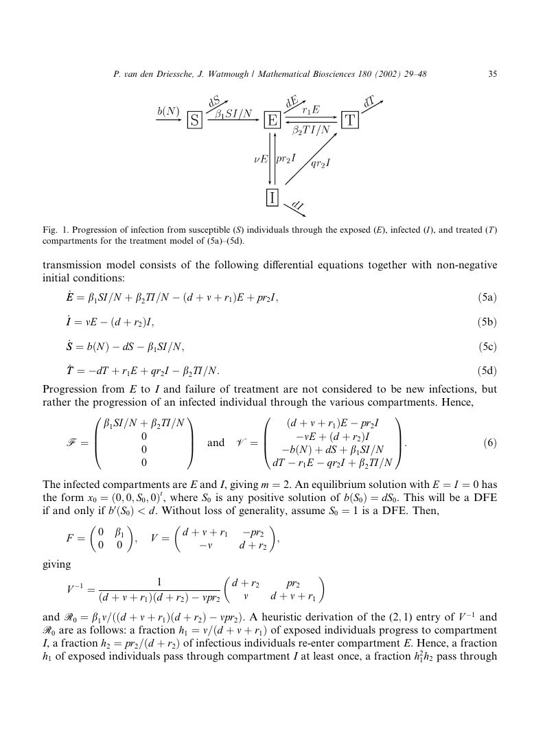
berculosis (S), exposed individuals (E), infectious individuals (I) and treated individuals (T ). The
dynamics are illustrated in Fig. 1. Susceptible and treated individuals enter the exposed com-
partment at rates b1I=N and b2I=N , respectively, where N ¼ E þ I þ S þ T . Exposed individuals
progress to the infectious compartment at the rate m. All newborns are susceptible, and all indi-
viduals die at the rate d > 0. Thus, the core of the model is an SEI model using standard inci-
dence. The treatment rates are r1 for exposed individuals and r2 for infectious individuals.
However, only a fraction q of the treatments of infectious individuals are successful. Unsuc-
cessfully treated infectious individuals re-enter the exposed compartment (p ¼ 1 � q). The disease
�
P. van den Driessche, J. Watmough / Mathematical Biosciences 180 (2002) 29–48
35
Fig. 1. Progression of infection from susceptible (S) individuals through the exposed (E), infected (I), and treated (T )
compartments for the treatment model of (5a)–(5d).
transmission model consists of the following differential equations together with non-negative
initial conditions:
_EE ¼ b1SI=N þ b2TI=N � ðd þ m þ r1ÞE þ pr2I;
_II ¼ mE � ðd þ r2ÞI;
_SS ¼ bðNÞ � dS � b1SI=N ;
_TT ¼ �dT þ r1E þ qr2I � b2TI=N :
ð5aÞ
ð5bÞ
ð5cÞ
ð5dÞ
Progression from E to I and failure of treatment are not considered to be new infections, but
rather the progression of an infected individual through the various compartments. Hence,
F ¼
b1SI=N þ b2TI=N
0
0
0
0
BB@
�
1
CCA and V ¼
0
BB@
1
CCA:
ðd þ m þ r1ÞE � pr2I
�mE þ ðd þ r2ÞI
�bðNÞ þ dS þ b1SI=N
dT � r1E � qr2I þ b2TI=N
�
ð6Þ
The infected compartments are E and I, giving m ¼ 2. An equilibrium solution with E ¼ I ¼ 0 has
the form x0 ¼ ð0; 0; S0; 0Þt, where S0 is any positive solution of bðS0Þ ¼ dS0. This will be a DFE
if and only if b0ðS0Þ < d. Without loss of generality, assume S0 ¼ 1 is a DFE. Then,
�
�
F ¼ 0 b1
0
0
;
giving
V ¼ d þ m þ r1 �pr2
d þ r2
�m
;
�
�
V �1 ¼
1
ðd þ m þ r1Þðd þ r2Þ � mpr2
d þ r2
m
pr2
d þ m þ r1
and R0 ¼ b1m=ððd þ m þ r1Þðd þ r2Þ � mpr2Þ. A heuristic derivation of the (2; 1) entry of V �1 and
R0 are as follows: a fraction h1 ¼ m=ðd þ m þ r1Þ of exposed individuals progress to compartment
I, a fraction h2 ¼ pr2=ðd þ r2Þ of infectious individuals re-enter compartment E. Hence, a fraction
h1 of exposed individuals pass through compartment I at least once, a fraction h2
1h2 pass through
�
36
P. van den Driessche, J. Watmough / Mathematical Biosciences 180 (2002) 29–48
2
1hk�1
pass through at least k times, spending an average of s ¼
at least twice, and a fraction hk
1=ðd þ r2Þ time units in compartment I on each pass. Thus, an individual introduced into com-
1h2 þ ���Þ ¼ sh1=ð1 � h1h2Þ ¼ m=ððd þ m þ r1Þðd þ r2Þ�
partment E spends, on average, sðh1 þ h2
mpr2Þ time units in compartment I over its expected lifetime. Multiplying this by b1 gives R0.
The model without treatment (r1 ¼ r2 ¼ 0) is an SEI model with R0 ¼ b1m=ðdðd þ mÞÞ. The
interpretation of R0 for this case is simpler. Only a fraction m=ðd þ mÞ of exposed individuals
progress from compartment E to compartment I, and individuals entering compartment I spend,
on average, 1=d time units there.
Although conditions (A1)–(A5) do not restrict the decomposition of fiðxÞ to a single choice for
Fi, only one such choice is epidemiologically correct. Different choices for the function F lead to
different values for the spectral radius of FV �1, as shown in Table 1. In column (a), treatment
failure is considered to be a new infection and in column (b), both treatment failure and pro-
gression to infectiousness are considered new infections. In each case the condition qðFV �1Þ < 1
yields the same portion of parameter space. Thus, qðFV �1Þ is a threshold parameter in both cases.
The difference between the numbers lies in the epidemiological interpretation rather than the
mathematical analysis. For example, in column (a), the infection rate is b1 þ pr2 and an exposed
individual is expected to spend m=ððd þ m þ r1Þðd þ r2ÞÞ time units in compartment I. However,
this reasoning is biologically flawed since treatment failure does not give rise to a newly infected
individual.
Table 1
Decomposition of f leading to alternative thresholds
0
BB@
0
BB@
(a)
b1SI=N þ b2TI=N þ pr2I
0
0
0
ðd þ m þ r1ÞE
�mE þ ðd þ r2ÞI
�bðNÞ þ dS þ b1SI=N
�
�
dT � r1E � qr2I þ b2TI=N
�
�
0 b1 þ pr2
0
0
d þ m þ r1
0
d þ r2
�m
b1m þ pr2m
ðd þ m þ r1Þðd þ r2Þ
F
V
F
V
q(FV �1)
1
CCA
1
CCA
1
CCA
1
CCA
0
BB@
0
BB@
(b)
b1SI=N þ b2TI=N þ pr2I
mE
0
0
ðd þ r2ÞI
ðd þ m þ r1ÞE
�bðNÞ þ dS þ b1SI=N
�
�
dT � r1E � qr2I þ b2TI=N
�
�
d þ m þ r1
ffiffiffiffiffiffiffiffiffiffiffiffiffiffiffiffiffiffiffiffiffiffiffiffiffiffiffiffiffiffiffiffiffiffiffiffiffiffiffiffi
s
d þ r2
0 b1 þ pr2
m
0
0
0
b1m þ pr2m
ðd þ m þ r1Þðd þ r2Þ
�


 2023年江西萍乡中考道德与法治真题及答案.doc
 2012年重庆南川中考生物真题及答案.doc
 2013年江西师范大学地理学综合及文艺理论基础考研真题.doc
 2020年四川甘孜小升初语文真题及答案I卷.doc
 2020年注册岩土工程师专业基础考试真题及答案.doc
 2023-2024学年福建省厦门市九年级上学期数学月考试题及答案.doc
 2021-2022学年辽宁省沈阳市大东区九年级上学期语文期末试题及答案.doc
 2022-2023学年北京东城区初三第一学期物理期末试卷及答案.doc
 2018上半年江西教师资格初中地理学科知识与教学能力真题及答案.doc
 2012年河北国家公务员申论考试真题及答案-省级.doc
 2020-2021学年江苏省扬州市江都区邵樊片九年级上学期数学第一次质量检测试题及答案.doc
 2022下半年黑龙江教师资格证中学综合素质真题及答案.doc