自监督学习：生成和对比方法综述.pdf

发布时间：2022-05-31 发布人：admin 分类：说明书资料大小：7.47M 资料格式：pdf 举报版权申诉

syp_net-12535924-4744300845198320800.pdf-第1页.png

第1页 / 共20页

syp_net-12535924-4744300845198320800.pdf-第2页.png

第2页 / 共20页

syp_net-12535924-4744300845198320800.pdf-第3页.png

第3页 / 共20页

syp_net-12535924-4744300845198320800.pdf-第4页.png

第4页 / 共20页

syp_net-12535924-4744300845198320800.pdf-第5页.png

第5页 / 共20页

syp_net-12535924-4744300845198320800.pdf-第6页.png

第6页 / 共20页

syp_net-12535924-4744300845198320800.pdf-第7页.png

第7页 / 共20页

syp_net-12535924-4744300845198320800.pdf-第8页.png

第8页 / 共20页

1 Introduction

2 Background

2.1 Representation Learning in NLP

2.2 Representation Learning in CV

2.3 Representation Learning on Graphs

3 Generative Self-supervised Learning

3.1 Auto-regressive (AR) Model

3.2 Flow-based Model

3.3 Auto-encoding (AE) Model

3.3.1 Basic AE Model

3.3.2 Context Prediction Model (CPM)

3.3.3 Denoising AE Model

3.3.4 Variational AE Model

3.4 Hybrid Generative Models

3.4.1 Combining AR and AE Model.

3.4.2 Combining AE and Flow-based Models

4 Contrastive Self-supervised Learning

4.1 Context-Instance Contrast

4.1.1 Predict Relative Position

4.1.2 Maximize Mutual Information

4.2 Context-Context Contrast

4.2.1 Cluster-based Discrimination

4.2.2 Instance Discrimination

5 Generative-Contrastive (Adversarial) Self-supervised Learning

5.1 Why Generative-Contrastive (Adversarial)?

5.2 Generate with Complete Input

5.3 Recover with Partial Input

5.4 Pre-trained Language Model

5.5 Graph Learning

5.6 Domain Adaptation and Multi-modality Representation

6 Theory behind Self-supervised Learning

6.1 GAN

6.1.1 Divergence Matching

6.1.2 Disentangled Representation

6.2 Maximizing Lower Bound

6.2.1 Evidence Lower Bound

6.2.2 Mutual Information

6.3 Contrastive Self-supervised Representation Learning

7 Discussions and Future Directions

References

Biographies

Xiao Liu

Fanjin Zhang

Zhenyu Hou

Li Mian

Zhaoyu Wang

Jing Zhang

Jie Tang

0 2 0 2 n u J 6 1 ] G L . s c [ 2 v 8 1 2 8 0 . 6 0 0 2 : v i X r a Self-supervised Learning: Generative or Contrastive Xiao Liu, Fanjin Zhang, Zhenyu Hou, Li Mian, Zhaoyu Wang, Jing Zhang, Jie Tang, Senior Member 1 Abstract—Deep supervised learning has achieved great success in the last decade. However, its deﬁciencies of dependence on manual labels and vulnerability to attacks have driven people to explore a better solution. As an alternative, self-supervised learning attracts many researchers for its soaring performance on representation learning in the last several years. Self-supervised representation learning leverages input data itself as supervision and beneﬁts almost all types of downstream tasks. In this survey, we take a look into new self-supervised learning methods for representation in computer vision, natural language processing, and graph learning. We comprehensively review the existing empirical methods and summarize them into three main categories according to their objectives: generative, contrastive, and generative-contrastive (adversarial). We further investigate related theoretical analysis work to provide deeper thoughts on how self-supervised learning works. Finally, we brieﬂy discuss open problems and future directions for self-supervised learning. Index Terms—Self-supervised Learning, Generative Model, Contrastive Learning, Deep Learning ! 1 INTRODUCTION D eep neural networks [77] have shown outstanding performance on various machine learning tasks, es- pecially on supervised learning in computer vision (image classiﬁcation [32], [54], [59], semantic segmentation [45], [85]), natural language processing (pre-trained language models [33], [74], [84], [149], sentiment analysis [83], question answering [5], [35], [111], [150] etc.) and graph learning (node classiﬁcation [58], [70], [106], [138], graph classiﬁcation [7], [123], [155] etc.). Generally, the supervised learning is trained over a speciﬁc task with a large manually labeled dataset which is randomly divided into training, validatiton and test sets. However, supervised learning is meeting its bottleneck. It not only relies heavily on expensive manual labeling but also suffers from generalization error, spurious cor- relations, and adversarial attacks. We expect the neural network to learn more with fewer labels, fewer samples, or fewer trials. As a promising candidate, self-supervised learning has drawn massive attention for its fantastic data efﬁciency and generalization ability, with many state-of- the-art models following this paradigm. In this survey, we will take a comprehensive look at the development of the recent self-supervised learning models and discuss their theoretical soundness, including frameworks such as Pre- trained Language Models (PTM), Generative Adversarial • • Xiao Liu, Fanjin Zhang, and Zhengyu Hou are with the Department of Computer Science and Technology, Tsinghua University, Beijing, China. E-mail: liuxiao17@mails.tsinghua.edu.cn, zfj17@mails.tsinghua.edu.cn, hzy17@mails.tsinghua.edu.cn Jie Tang is with the Department of Computer Science and Technology, Tsinghua University, and Tsinghua National Laboratory for Information Science and Technology (TNList), Beijing, China, 100084. E-mail: jietang@tsinghua.edu.cn, corresponding author Li Mian is with the Beijing Institute of Technonlogy, Beijing, China. Email: 1120161659@bit.edu.cn • • Zhaoyu Wang is with the Anhui University, Anhui, China. • Email: wzy950507@163.com Jing Zhang is with the Renming University of China, Beijing, China. 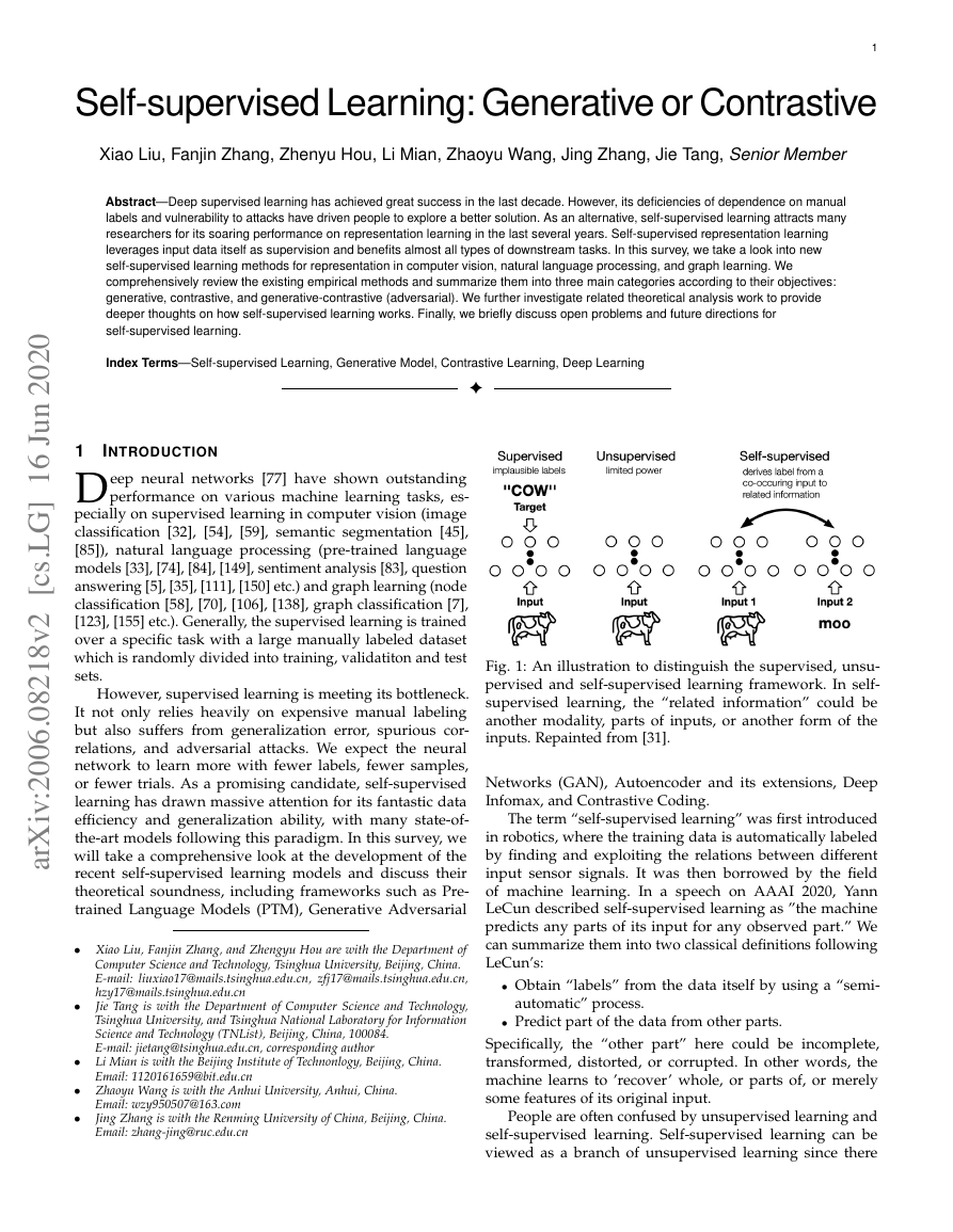Email: zhang-jing@ruc.edu.cn Fig. 1: An illustration to distinguish the supervised, unsu- pervised and self-supervised learning framework. In self- supervised learning, the “related information” could be another modality, parts of inputs, or another form of the inputs. Repainted from [31]. Networks (GAN), Autoencoder and its extensions, Deep Infomax, and Contrastive Coding. The term “self-supervised learning” was ﬁrst introduced in robotics, where the training data is automatically labeled by ﬁnding and exploiting the relations between different input sensor signals. It was then borrowed by the ﬁeld of machine learning. In a speech on AAAI 2020, Yann LeCun described self-supervised learning as ”the machine predicts any parts of its input for any observed part.” We can summarize them into two classical deﬁnitions following LeCun’s: • Obtain “labels” from the data itself by using a “semi- automatic” process. • Predict part of the data from other parts. Speciﬁcally, the “other part” here could be incomplete, transformed, distorted, or corrupted. In other words, the machine learns to ’recover’ whole, or parts of, or merely some features of its original input. People are often confused by unsupervised learning and self-supervised learning. Self-supervised learning can be viewed as a branch of unsupervised learning since there

is no manual label involved. However, narrowly speaking, unsupervised learning concentrates on detecting speciﬁc data patterns, such as clustering, community discovery, or anomaly detection, while self-supervised learning aims at recovering, which is still in the paradigm of supervised set- tings. Figure 1 provides a vivid explanation of the differences between them. 2 There exist several comprehensive reviews related to Pre- trained Language Models [107], Generative Adversarial Net- works [142], Autoencoder and contrastive learning for visual representation [64]. However, none of them concentrates on the inspiring idea of self-supervised learning that illustrates researchers and models in many ﬁelds. In this work, we collect studies from natural language processing, computer vision, and graph learning in recent years to present an up- to-date and comprehensive retrospective on the frontier of self-supervised learning. To sum up, our contributions are: • We provide a detailed and up-to-date review of self- supervised learning for representation. We introduce the background knowledge, models with variants, and important frameworks. One can easily grasp the frontier ideas of self-supervised learning. • We categorize self-supervised learning models into generative, contrastive, and generative-contrastive (ad- versarial), with particular genres inner each one. We demonstrate the pros and cons of each category and discuss the recent attempt to shift from generative to contrastive. • We examine the theoretical soundness of self-supervised learning methods and show how it can beneﬁt the downstream supervised learning tasks. • We identify several open problems in this ﬁeld, analyze the limitations and boundaries, and discuss the future direction for self-supervised representation learning. We organize the survey as follows. In Section 2, we introduce the preliminary knowledge for new computer vision, natural language processing, and graph learning. From Section 3 to Section 5, we will introduce the empirical self-supervised learning methods utilizing generative, con- trastive and generative-contrastive objectives. In Section 6, we investigate the theoretical basis behind the success of self- supervised learning and its merits and drawbacks. In Section 7, we discuss the open problems and future directions in this ﬁeld. 2 BACKGROUND 2.1 Representation Learning in NLP Pre-trained word representations are key components in natural language processing tasks. Word embedding is to represent words as low-dimensional real-valued vectors. There are two kinds of word embeddings: non-contextual and contextual embeddings. Non-contextual Embeddings does not consider the con- text information of the token; that is, these models only map the token into a distributed embedding space. Thus, for each word x in the vocabulary V , embedding will assign it a speciﬁc vector.ex ∈ Rd, where d is the dimension of the embedding. These embeddings can not model complex characteristics of word use and polysemous. 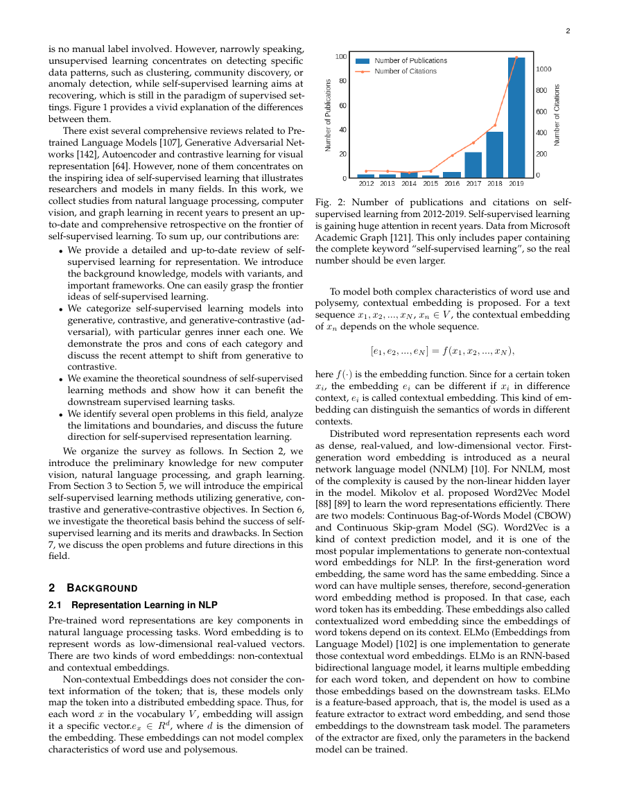Fig. 2: Number of publications and citations on self- supervised learning from 2012-2019. Self-supervised learning is gaining huge attention in recent years. Data from Microsoft Academic Graph [121]. This only includes paper containing the complete keyword “self-supervised learning”, so the real number should be even larger. To model both complex characteristics of word use and polysemy, contextual embedding is proposed. For a text sequence x1, x2, ..., xN , xn ∈ V , the contextual embedding of xn depends on the whole sequence. [e1, e2, ..., eN ] = f (x1, x2, ..., xN ), here f (·) is the embedding function. Since for a certain token xi, the embedding ei can be different if xi in difference context, ei is called contextual embedding. This kind of em- bedding can distinguish the semantics of words in different contexts. Distributed word representation represents each word as dense, real-valued, and low-dimensional vector. First- generation word embedding is introduced as a neural network language model (NNLM) [10]. For NNLM, most of the complexity is caused by the non-linear hidden layer in the model. Mikolov et al. proposed Word2Vec Model [88] [89] to learn the word representations efﬁciently. There are two models: Continuous Bag-of-Words Model (CBOW) and Continuous Skip-gram Model (SG). Word2Vec is a kind of context prediction model, and it is one of the most popular implementations to generate non-contextual word embeddings for NLP. In the ﬁrst-generation word embedding, the same word has the same embedding. Since a word can have multiple senses, therefore, second-generation word embedding method is proposed. In that case, each word token has its embedding. These embeddings also called contextualized word embedding since the embeddings of word tokens depend on its context. ELMo (Embeddings from Language Model) [102] is one implementation to generate those contextual word embeddings. ELMo is an RNN-based bidirectional language model, it learns multiple embedding for each word token, and dependent on how to combine those embeddings based on the downstream tasks. ELMo is a feature-based approach, that is, the model is used as a feature extractor to extract word embedding, and send those embeddings to the downstream task model. The parameters of the extractor are ﬁxed, only the parameters in the backend model can be trained.

Recently, BERT (Bidirectional Encoder Representations from Transformers) [33] bring large improvements on 11 NLP tasks. Different from feature-based approaches like ELMo, BERT is a ﬁne-tuned approach. The model is ﬁrst pre- trained on a large number of corpora through self-supervised learning, then ﬁne-tuned with labeled data. As the name showed, BERT is an encoder of the transformer, in the training stage, BERT masked some tokens in the sentence, then training to predict the masked word. When use BERT, initialized the BERT model with pre-trained weights, and ﬁne-tune the pre-trained model to solve downstream tasks. 2.2 Representation Learning in CV Computer vision is one of the greatest beneﬁted ﬁelds thanks to deep learning. In the past few years, researchers have developed a range of efﬁcient network architectures for supervised tasks. For self-supervised tasks, many of them are also proved to be useful. In this section, we introduce ResNet architecture [54], which is the backbone of a large part of the self-supervised techniques for visual representation models. Since AlexNet [73], CNN architecture is going deeper and deeper. While AlexNet had only ﬁve convolutional layers, the VGG network [120]and GoogleNet (also codenamed Inception v1) [127] had 19 and 22 layers respectively. Evidence [120], [127] reveals that network depth is of crucial importance, and driven by its signiﬁcance of depth, a question arises: Is learning better networks as easy as stacking more layers? An obstacle to answering this question was the notorious problem of vanishing/exploding gradients [12], which hamper convergence from the beginning. This problem, however, has been addressed mainly by normal- ized initialization [79], [116]and intermediate normalization layers [61], which enable networks with tens of layers to start converging for stochastic gradient descent (SGD) with backpropagation [78]. When deeper networks can start converging, a degra- dation problem has been exposed: with the network depth increasing, accuracy becomes saturated (which might be unsurprising) and then degrades rapidly. Unexpectedly, such degradation is not caused by overﬁtting, and adding more layers to a suitably deep model will lead to higher training error Residual neural network (ResNet), proposed by He et al. [54], effectively resolved this problem. Instead of asking every few stacked layers to directly learn a desired underlying mapping, authors of [54] design a residual mapping architec- ture ResNet. The core idea of ResNet is the introduction of shortcut connections(Fig. 2), which are those skipping over one or more layers. 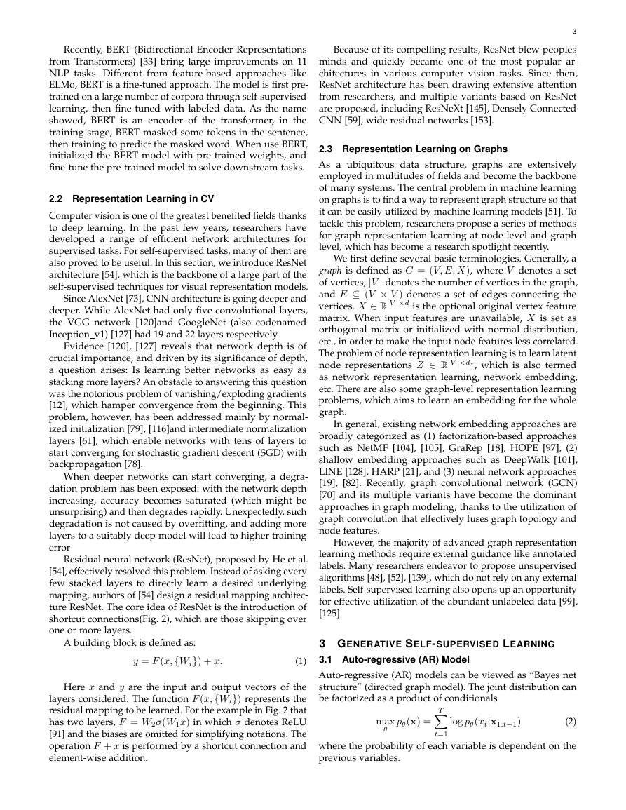A building block is deﬁned as: y = F (x,{Wi}) + x. (1) Here x and y are the input and output vectors of the layers considered. The function F (x,{Wi}) represents the residual mapping to be learned. For the example in Fig. 2 that has two layers, F = W2σ(W1x) in which σ denotes ReLU [91] and the biases are omitted for simplifying notations. The operation F + x is performed by a shortcut connection and element-wise addition. 3 Because of its compelling results, ResNet blew peoples minds and quickly became one of the most popular ar- chitectures in various computer vision tasks. Since then, ResNet architecture has been drawing extensive attention from researchers, and multiple variants based on ResNet are proposed, including ResNeXt [145], Densely Connected CNN [59], wide residual networks [153]. 2.3 Representation Learning on Graphs As a ubiquitous data structure, graphs are extensively employed in multitudes of ﬁelds and become the backbone of many systems. The central problem in machine learning on graphs is to ﬁnd a way to represent graph structure so that it can be easily utilized by machine learning models [51]. To tackle this problem, researchers propose a series of methods for graph representation learning at node level and graph level, which has become a research spotlight recently. We ﬁrst deﬁne several basic terminologies. Generally, a graph is deﬁned as G = (V, E, X), where V denotes a set of vertices, |V | denotes the number of vertices in the graph, and E ⊆ (V × V ) denotes a set of edges connecting the vertices. X ∈ R|V |×d is the optional original vertex feature matrix. When input features are unavailable, X is set as orthogonal matrix or initialized with normal distribution, etc., in order to make the input node features less correlated. The problem of node representation learning is to learn latent node representations Z ∈ R|V |×dz , which is also termed as network representation learning, network embedding, etc. There are also some graph-level representation learning problems, which aims to learn an embedding for the whole graph. In general, existing network embedding approaches are broadly categorized as (1) factorization-based approaches such as NetMF [104], [105], GraRep [18], HOPE [97], (2) shallow embedding approaches such as DeepWalk [101], LINE [128], HARP [21], and (3) neural network approaches [19], [82]. Recently, graph convolutional network (GCN) [70] and its multiple variants have become the dominant approaches in graph modeling, thanks to the utilization of graph convolution that effectively fuses graph topology and node features. However, the majority of advanced graph representation learning methods require external guidance like annotated labels. Many researchers endeavor to propose unsupervised algorithms [48], [52], [139], which do not rely on any external labels. Self-supervised learning also opens up an opportunity for effective utilization of the abundant unlabeled data [99], [125]. 3 GENERATIVE SELF-SUPERVISED LEARNING 3.1 Auto-regressive (AR) Model Auto-regressive (AR) models can be viewed as “Bayes net structure” (directed graph model). The joint distribution can be factorized as a product of conditionals T t=1 max θ pθ(x) = log pθ(xt|x1:t−1) (2) where the probability of each variable is dependent on the previous variables.

Model word2vec [88], [89] FastText [15] NICE [36] RealNVP [37] Glow [68] FOS GPT/GPT-2 [109], [110] NLP PixelCNN [134], [136] CV CV CV CV NLP NLP Graph Graph NLP NLP NLP SpanBERT [65] ALBERT [74] DeepWalk-based [47], [101], [128] VGAE [71] BERT [33] ERNIE [126] VQ-VAE 2 [112] XLNet [149] RelativePosition [38] CDJP [67] PIRL [90] RotNet [44] Deep InfoMax [55] AMDIM [6] CPC [96] InfoWord [72] DGI [139] InfoGraph [123] S2GRL [99] Pre-trained GNN [57] DeepCluster [20] Local Aggregation [160] ClusterFit [147] InstDisc [144] CMC [130] MoCo [53] MoCo v2 [25] SimCLR [22] GCC [63] GAN [46] Adversarial AE [86] BiGAN/ALI [39], [42] BigBiGAN [40] Colorization [75] Inpainting [98] Super-resolution [80] ELECTRA [27] WKLM [146] ANE [29] GraphGAN [140] GraphSGAN [34] NLP CV NLP CV CV CV CV CV CV CV NLP Graph Graph Graph Graph CV CV CV CV CV CV CV CV Graph CV CV CV CV CV CV CV NLP NLP Graph Graph Graph Type Generator G G G G G G G G G G G G G G G C C C C C C C C C C C C C C C C C C C C C G-C G-C G-C G-C G-C G-C G-C G-C G-C G-C G-C G-C AR AR Flow based AE AE AE AE AE AE AE AE AE AE+AR - - - - - - - - - - - - - - - - - - - - - AE AE AE AE AE AE AE AE AE AE AE AE Self-supervision Following words Following pixels Pretext Task Next word prediction Next pixel prediction Whole image Image reconstruction Context words CBOW & SkipGram CBOW Graph edges Link prediction Masked words Sentence topic Masked words Masked words Sentence order Masked words Sentence topic Whole image Masked words Spatial relations (Context-Instance) Masked language model, Next senetence prediction Masked language model Masked language model, Sentence order prediction Masked language model, Next senetence prediction Image reconstruction Permutation language model Relative postion prediction Jigsaw + Inpainting + Colorization Jigsaw Rotation Prediction Belonging (Context-Instance) MI Maximization Belonging Node attributes MI maximization, Masked attribute prediction Similarity (Context-Context) Cluster discrimination Identity (Context-Context) Instance discrimination Whole image Image reconstruction Image color Parts of images Details of images Masked words Masked entities Graph edges Graph nodes Colorization Inpainting Super-resolution Replaced token detection Replaced entity detection Link prediction Node classiﬁcation Hard NS - - - - - × × × × - - - Hard PS - - - - - × × × × - - - - - - - × × - × × × × × × × - - - × × × × × × - - - - - - - - - - - - - - × - × × × × × × × - - - × × - - - - - - - × × - - - 4 NS strategy - - - - - End-to-end End-to-end End-to-end End-to-end - - - - - - - End-to-end Memory bank - End-to-end End-to-end End-to-end End-to-end End-to-end End-to-end (batch-wise) End-to-end End-to-end - - - Memory bank End-to-end Momentum Momentum End-to-end (batch-wise) Momentum - - - - - - - End-to-end End-to-end - - - 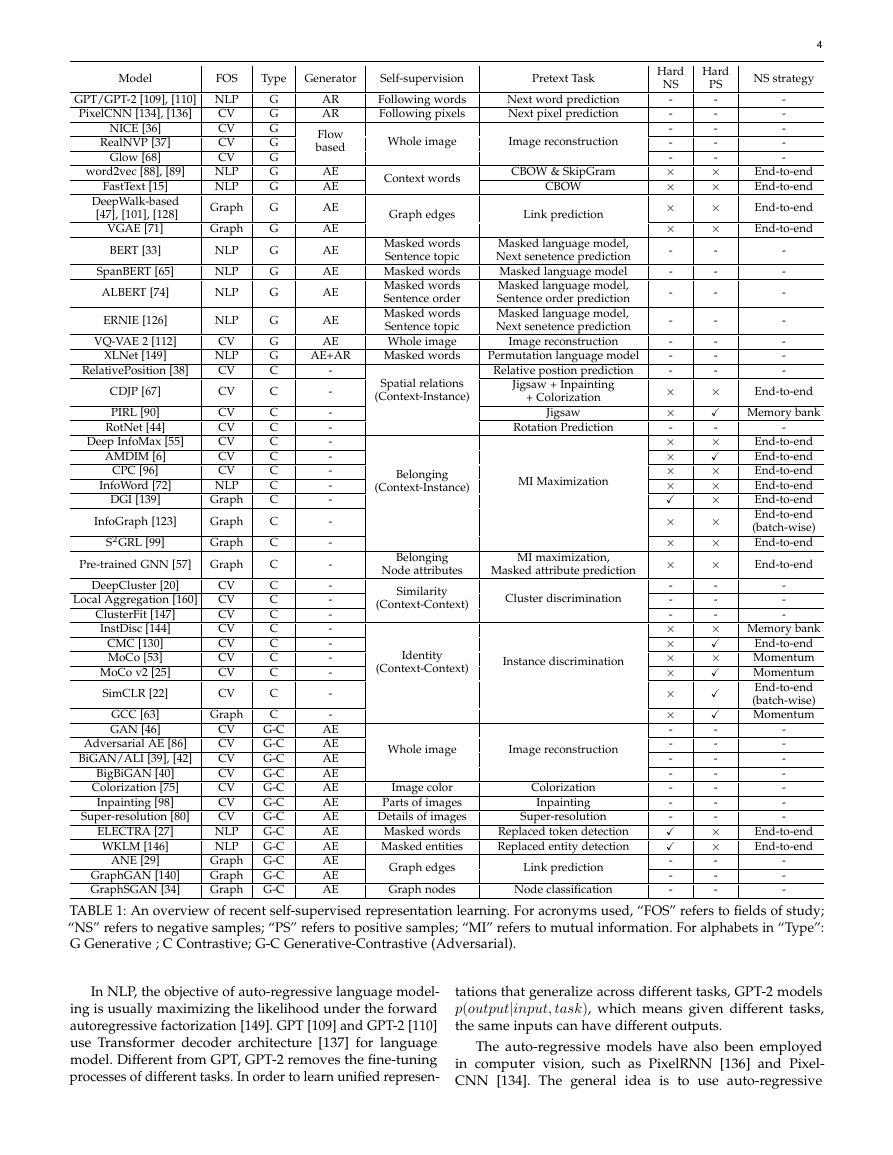TABLE 1: An overview of recent self-supervised representation learning. For acronyms used, “FOS” refers to ﬁelds of study; “NS” refers to negative samples; “PS” refers to positive samples; “MI” refers to mutual information. For alphabets in “Type”: G Generative ; C Contrastive; G-C Generative-Contrastive (Adversarial). In NLP, the objective of auto-regressive language model- ing is usually maximizing the likelihood under the forward autoregressive factorization [149]. GPT [109] and GPT-2 [110] use Transformer decoder architecture [137] for language model. Different from GPT, GPT-2 removes the ﬁne-tuning processes of different tasks. In order to learn uniﬁed represen- tations that generalize across different tasks, GPT-2 models p(output|input, task), which means given different tasks, the same inputs can have different outputs. The auto-regressive models have also been employed in computer vision, such as PixelRNN [136] and Pixel- CNN [134]. The general idea is to use auto-regressive

methods to model images pixel by pixel. For example, the lower (right) pixels are generated by conditioning on the upper (left) pixels. The pixel distributions of PixelRNN and PixelCNN are modeled by RNN and CNN, respectively. For 2D images, auto-regressive models can only factorize probabilities according to speciﬁc directions (such as right and down). Therefore, masked ﬁlters are employed in CNN architecture. Furthermore, two convolutional networks are combined to remove the blind spot in images. Based on PixelCNN, WaveNet [133] – a generative model for raw audio was proposed. In order to deal with long-range temporal de- pendencies, dilated causal convolutions are developed to improve the receptive ﬁeld. Moreover, Gated Residual blocks and skip connections are employed to empower better expressivity. The auto-regressive models can also be applied to graph domain, such as for graph generation problem. You et al. [152] propose GraphRNN to generate realistic graphs with deep auto-regressive models. They decompose the graph generation process into a sequence generation of nodes and edges, conditioned on the graph generated so far. The objective of GraphRNN is deﬁned as the likelihood of the observed graph generation sequences. GraphRNN can be viewed as a hierarchical model, where a graph-level RNN maintains the state of the graph and generates new nodes, while an edge-level RNN generates new edges based on the current graph state. After that, MRNN [103] and GCPN [151] are proposed as auto-regressive approaches. MRNN and GCPN both use a reinforcement learning framework to generate molecule graphs through optimizing domain-speciﬁc rewards. However, MRNN mainly uses RNN-based networks for state representations, but GCPN employs GCN-based encoder networks. The advantage of auto-regressive models is that it can model the context dependency well. However, one shortcom- ing of the AR model is that the token at each position can only access its context from one direction. 3.2 Flow-based Model The goal of ﬂow-based models is to estimate complex high- dimensional densities p(x) from data. However, directly formalizing the densities are difﬁcult. Generally, ﬂow-based models ﬁrst deﬁne a latent variable z which follows a known distribution pZ(z). Then deﬁne z = fθ(x), where fθ is an invertible and differentiable function. The goal is to learn the transformation between x and z so that the density of x can be depicted. According to the integral rule, pθ(x)dx = p(z)dz. Therefore, the densities of x and z satisﬁes: ∂x ∂fθ(x) ∂fθ ∂x i (x(i)) θ + log (3) (4) pθ(x) = p(fθ(x)) and the objective is maximum likelihood: i max θ log pθ(x(i)) = max log pZ(fθ(x(i))) The advantage of ﬂow-based models is that the mapping between x and z is invertible. However, it also requires 5 that x and z must have the same dimension. fθ needs to be carefully designed since it should be invertible and the Jacobian determinant in Eq. (3) should also be calculated easily. NICE [36] and RealNVP [37] design afﬁne coupling layer to parameterize fθ. The core idea is to split x into two blocks (x1, x2) and apply a transformation from (x1, x2) to (z1, z2) in an auto-regressive manner, that is z1 = x1 and z2 = x2 + m(x1). More recently, Glow [68] was proposed and it introduces invertible 1× 1 convolutions and simpliﬁes RealNVP. 3.3 Auto-encoding (AE) Model The goal of the auto-encoding model is to reconstruct (part of) inputs from (corrupted) inputs. 3.3.1 Basic AE Model Autoencoder (AE) was ﬁrst introduced in [8] for pre-training in ANNs. Before Autoencoder, Restricted Boltzmann Ma- chine (RBM) [122] can also be viewed as a special “autoen- coder”. RBM is an undirected graphical model, and it only contains two layers: visible layer and hidden layer. The objective of RBM is to minimize the difference between the marginal distribution of models and data distributions. In contrast, autoencoder can be regarded as a directed graphical model, and it can be trained more easily. Autoencoder is typically for dimensionality reduction. Generally, autoen- coder is a feedforward neural network trained to produce its input at the output layer. AE is comprised of an encoder network h = fenc(x) and a decoder network x = fdec(h). The objective of AE is to make x and x as similar as possible (such as through mean-square error). It can be shown that linear autoencoder corresponds to PCA. Sometimes the number of hidden units is greater than the number of input units, and some interesting structures can be discovered by imposing sparsity constraints on the hidden units [92]. 3.3.2 Context Prediction Model (CPM) The idea of the Context Prediction Model (CPM) is predicting contextual information based on inputs. In NLP, when it comes to SSL on word embedding, CBOW, and Skip-Gram [89] are pioneering works. CBOW aims to predict the input tokens based on context tokens. In contrast, Skip-Gram aims to predict context tokens based on input tokens. Usually, negative sampling is employed to ensure computational efﬁciency and scalability. Following CBOW architecture, FastText [15] is proposed by utilizing subword information. Inspired by the progress of word embedding models in NLP, many network embedding models are proposed based on a similar context prediction objective. Deepwalk [101] samples truncated random walks to learn latent node embed- ding based on the Skip-Gram model. It treats random walks as the equivalent of sentences. However, LINE [128] aims to generate neighbors based on current nodes. wij log p(vj|vi) O = − (5) (i,j)∈E where E denotes edge set, v denotes the node, wij represents the weight of edge (vi, vj). LINE also uses negative sampling to sample multiple negative edges to approximate the objective.

3.3.3 Denoising AE Model The idea of denoising autoencoder models is that represen- tation should be robust to the introduction of noise. The masked language model (MLM) can be regarded as a de- noising AE model because its input masks predicted tokens. To model text sequence, masked language model (MLM) randomly masks some of the tokens from the input, and then predict them based their context information [33], which is similar to the Cloze task [129]. Speciﬁcally, in BERT [33], a unique token [MASK] is introduced in the training process to mask some tokens. However, one shortcoming of this method is that there are no input [MASK] tokens for down-stream tasks. To mitigate this, the authors do not always replace the predicted tokens with [MASK] in training. Instead, they replace them with original words or random words with a small probability. There emerge some extensions of MLM. SpanBERT [65] chooses to mask continuous random spans rather than random tokens adopted by BERT. Moreover, it trains the span boundary representations to predict the masked spans, which is inspired by ideas in coreference resolution. ERNIE (Baidu) [126] masks entities or phrases to learn entity-level and phrase-level knowledge, which obtains good results in Chinese natural language processing tasks. Compared with the AR model, in MLM, the predicted tokens have access to contextual information from both sides. However, MLM assumes that the predicted tokens are independent of each other if the unmasked tokens are given. 3.3.4 Variational AE Model The variational auto-encoding model assumes that data are generated from underlying latent (unobserved) representa- tion. The posterior distribution over a set of unobserved variables Z = {z1, z2, ..., zn} given some data X is approxi- mated by a variational distribution, q(z|x). p(z|x) ≈ q(z|x) (6) In variational inference and evidence lower bound (ELBO) on the log-likelihood of data is maximized during training. log p(x) ≥ −DKL(q(z|x)||p(z)) + E∼q(z|x)[log p(x|z)] (7) where p(x) is evidence probability, p(z) is prior and p(x|z) is likelihood probability. The right-hand side of the above equation is called ELBO. From the auto-encoding perspective, the ﬁrst term of ELBO is a regularizer forcing the posterior to approximate the prior. The second term is the likelihood of reconstructing the original input data based on latent variables. Variational Autoencoders (VAE) [69] is one important example where variational inference is utilized. VAE assumes the prior p(z) and the approximate posterior q(z|x) both follow Gaussian distributions. Speciﬁcally, let p(z) ∼ N (0, 1). Furthermore, reparameterization trick is utilized for mod- eling approximate posterior q(z|x). Assume z ∼ N (µ, σ2), z = µ + σ where ∼ N (0, 1). Both µ and σ are parameter- ized by neural networks. Based on calculated latent variable z, decoder network is utilized to reconstruct the input data. Recently, a novel and powerful variational AE model called VQ-VAE [135] was proposed. 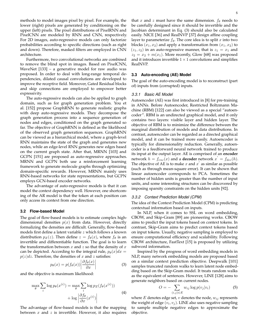VQ-VAE aims to learn 6 Fig. 3: Architecture of VQ-VAE [135]. Compared to VAE, the orginal hidden distribution is replaced with a quantized vec- tor dictionary. In addition, the prior distribution is replaced with a pre-trained PixelCNN that models the hierarchical features of images. Taken from [135] discrete latent variables, which is motivated since many modalities are inherently discrete, such as language, speech, and images. VQ-VAE relies on vector quantization (VQ) to learn the posterior distribution of discrete latent variables. Speciﬁcally, the discrete latent variables are calculated by the nearest neighbor lookup using a shared, learnable embedding table. In training, the gradients are approximated through straight-through estimator [11] as L(x, D(e)) = x−D(e)2 2+sg[E(x)]−e2 2+βsg[e]−E(x)2 2 (8) where e refers to the codebook, the operator sg refers to a stop-gradient operation that blocks gradients from ﬂowing into its argument, and β is a hyperparameter which controls the reluctance to change the code corresponding to the encoder output. More recently, researchers propose VQ-VAE-2 [112], which can generate versatile high-ﬁdelity images that rival that of state of the art Generative Adversarial Networks (GAN) BigGAN [16] on ImageNet [32]. First, the authors enlarge the scale and enhance the autoregressive priors by a powerful PixelCNN [134] prior. Additionally, they adopt a multi-scale hierarchical organization of VQ-VAE, which enables learning local information and global information of images separately. Nowadays, VAE and its variants have been widely used in the computer vision area, such as image representation learning, image generation, video generation. Variational auto-encoding models have also been em- ployed in node representation learning on graphs. For example, Variational graph auto-encoder (VGAE) [71] uses the same variational inference technique as VAE with graph convolutional networks (GCN) [70] as the encoder. Due to the uniqueness of graph-structured data, the objective of VGAE is to reconstruct the adjacency matrix of the graph by measuring node proximity. Zhu et al. [158] propose DVNE, a deep variational network embedding model in Wasserstein space. It learns Gaussian node embedding to model the uncertainty of nodes. 2-Wasserstein distance is used to measure the similarity between the distributions for its effectiveness in preserving network transitivity. vGraph [124] can perform node representation learning and community detection collaboratively through a generative variational inference framework. It assumes that each node can be gen- erated from a mixture of communities, and each community is deﬁned as a multinomial distribution over nodes.

7 design, such as valency check. Inspired by the recent progress of ﬂow-based models, it deﬁnes an invertible transformation from a base distribution (e.g., multivariate Gaussian) to a molecular graph structure. Additionally, Dequantization technique [56] is utilized to convert discrete data (including node types and edge types) into continuous data. 4 CONTRASTIVE SELF-SUPERVISED LEARNING From statistical perspective, machine learning models are categorized into two classes: generative model and discrim- inative model. Given the joint distribution P (X, Y ) of the input X and target Y , the generative model calculates the p(X|Y = y) by: p(X|Y = y) = p(X, Y ) p(Y = y) (10) while the discriminative model tries to model the P (Y |X = x) by: x p(Y, X = x) = p(X, Y ) p(Y |X = x) = p(X, Y ) p(X = x) = p(X, Y ) y p(Y = y, X) (11) Notice that most of the representation learning tasks hope to model relationships between x. Thus for a long time, people believe that the generative model is the only choice for representation learning. 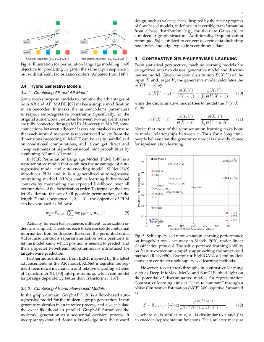Fig. 5: Self-supervised representation learning performance on ImageNet top-1 accuracy in March, 2020, under linear classiﬁcation protocol. The self-supervised learning’s ability on feature extraction is rapidly approaching the supervised method (ResNet50). Except for BigBiGAN, all the models above are contrastive self-supervised learning methods. However, recent breakthroughs in contrastive learning, such as Deep InfoMax, MoCo and SimCLR, shed light on the potential of discriminative models for representation. Contrastive learning aims at ”learn to compare” through a Noise Contrastive Estimation (NCE) [49] objective formatted as: L = Ex,x+,x− [−log( (12) where x+ is similar to x, x− is dissimilar to x and f is an encoder (representation function). 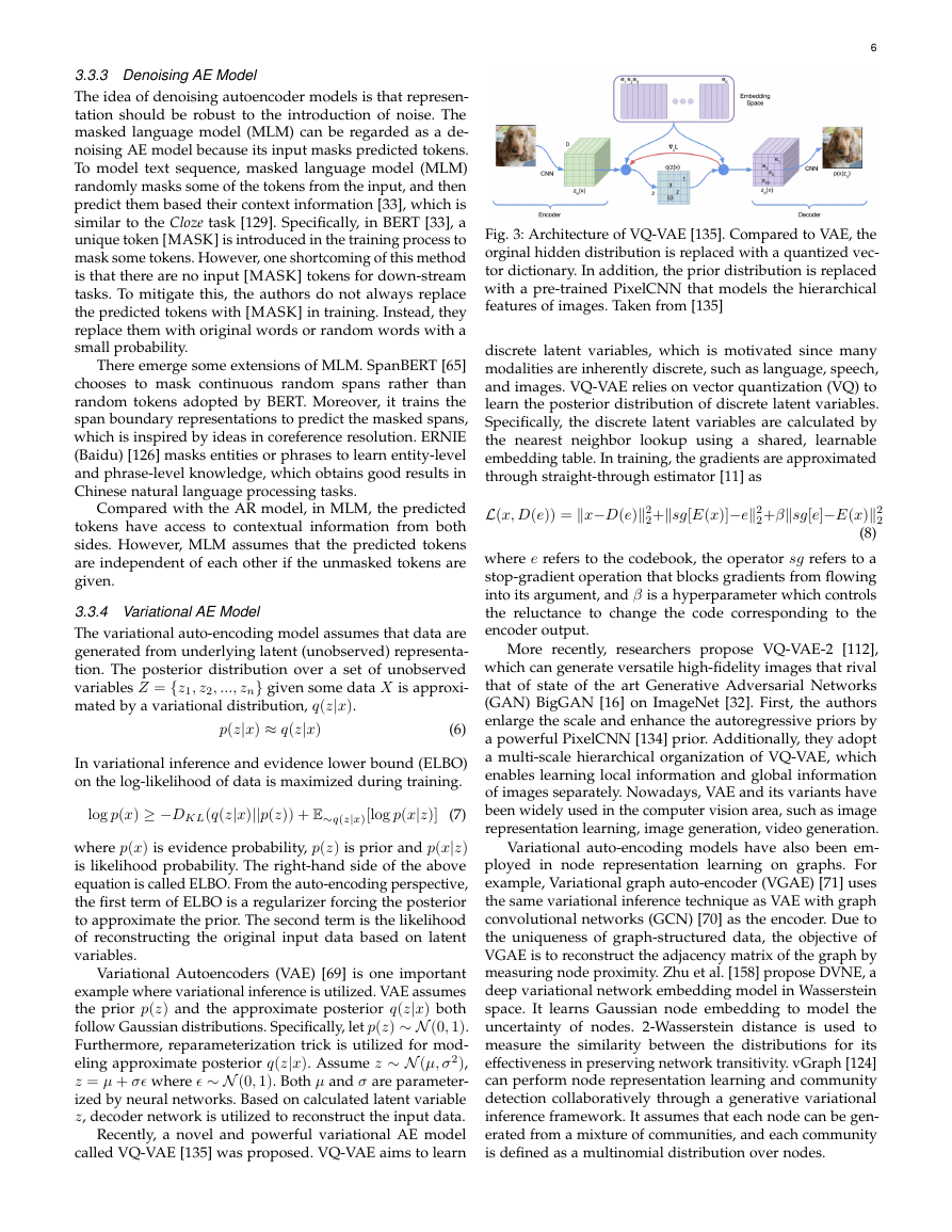The similarity measure ef (x)T f (x+) + ef (x)T f (x−) ef (x)T f (x+) ] Fig. 4: Illustration for permutation language modeling [149] objective for predicting x3 given the same input sequence x but with different factorization orders. Adpated from [149] 3.4 Hybrid Generative Models 3.4.1 Combining AR and AE Model. Some works propose models to combine the advantages of both AR and AE. MADE [87] makes a simple modiﬁcation to autoencoder. It masks the autoencoder’s parameters to respect auto-regressive constraints. Speciﬁcally, for the original autoencoder, neurons between two adjacent layers are fully-connected through MLPs. However, in MADE, some connections between adjacent layers are masked to ensure that each input dimension is reconstructed solely from the dimensions preceding it. MADE can be easily parallelized on conditional computations, and it can get direct and cheap estimates of high-dimensional joint probabilities by combining AE and AR models. In NLP, Permutation Language Model (PLM) [149] is a representative model that combines the advantage of auto- regressive model and auto-encoding model. XLNet [149] introduces PLM and it is a generalized auto-regressive pretraining method. XLNet enables learning bidirectional contexts by maximizing the expected likelihood over all permutations of the factorization order. To formalize the idea, let ZT denote the set of all possible permutations of the length-T index sequence [1, 2, ..., T ], the objective of PLM can be expressed as follows: Ez∼ZT [ max θ log pθ(xzt|xz

8 is initially introduced by BERT [33], where for a sentence, the model is asked to distinguish the right next sentence, and a randomly sampled one. However, some later work empirically proves that NSP helps little, even harm the performance. So in RoBERTa [84], the NSP loss is removed. To replace NSP, ALBERT [74] proposes Sentence Order Prediction (SOP) task. That is because, in NSP, the negative next sentence is sampled from other passages that may have different topics with the current one, turning the NSP into a far easier topic model problem. In SOP, two sentences that exchange their position are regarded as a negative sample, making the model concentrate on the coherence of the semantic meaning. 4.1.2 Maximize Mutual Information This kind of method derives from mutual information (MI) – a basic concept in statistics. Mutual information targets at modeling this association, and our objective is to maximize it. Generally, this kind of models optimize max g1∈G1,g2∈G1 I(g1(x1), g2(x2)) (14) where gi is the representation encoder, Gi is a class of encoders with some constraints and I(·,·) is a sample-based estimator for the real mutual information. In applications, MI is notorious for its hard computation. A common practice is to maximize I’s lower bound with an NCE objective. and encoder may vary from task to task, but the framework remains the same. With more dissimilar pairs involved, we have the InfoNCE [96] formulated as: L = Ex,x+,xk [−log( ef (x)T f (x+) +K ef (x)T f (x+) k=1 ef (x)T f (xk) ] (13) Here we divide recent contrastive learning frameworks into 2 types: context-instance contrast and instance-instance contrast. Both of them achieve amazing performance in downstream tasks, especially on classiﬁcation problems under the linear protocol. 4.1 Context-Instance Contrast The context-instance contrast, or so-called global-local contrast, focuses on modeling the belonging relationship between the local feature of a sample and its global context representation. When we learn the representation for a local feature, we hope it is associative to the representation of the global content, such as stripes to tigers, sentences to its paragraph, and nodes to their neighbors. There are two main types of Context-Instance Contrast: Predict Relative Position (PRP) and Maximize Mutual Infor- mation (MI). The differences between them are: • PRP focuses on learning relative positions between local components. The global context serves as an implicit requirement for predicting these relations (such as understanding what an elephant looks like is critical for predicting relative position between its head and tail). • MI focuses on learning the explicit belonging relation- ships between local parts and global context. The relative positions between local parts are ignored. 4.1.1 Predict Relative Position Many data contain rich spatial or sequential relations be- tween parts of it. For example, in image data such as Fig. 6, the elephant’s head is on the right of its tail. In text data, a sentence like ”Nice to meet you.” would probably be ahead of ”Nice to meet you, too.”. Various models regard recognizing relative positions between parts of it as the pretext task [64]. It could be relative positions of two patches from a sample [38], or to recover positions of shufﬂed segments of an image (solve jigsaw) [67], [93], [143], or to the rotation angle’s degree of an image [44]. A similar jigsaw technique is applied in PIRL [90] to augment the positive sample, but PIRL does not regard solving jigsaw and recovering spatial relation as its objective. 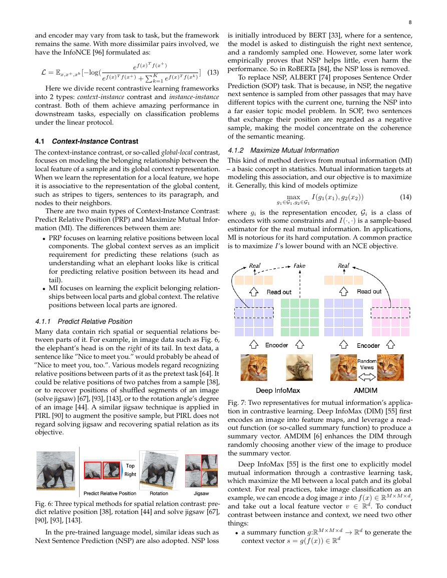Fig. 6: Three typical methods for spatial relation contrast: pre- dict relative position [38], rotation [44] and solve jigsaw [67], [90], [93], [143]. In the pre-trained language model, similar ideas such as Next Sentence Prediction (NSP) are also adopted. NSP loss Fig. 7: Two representatives for mutual information’s applica- tion in contrastive learning. Deep InfoMax (DIM) [55] ﬁrst encodes an image into feature maps, and leverage a read- out function (or so-called summary function) to produce a summary vector. AMDIM [6] enhances the DIM through randomly choosing another view of the image to produce the summary vector. Deep InfoMax [55] is the ﬁrst one to explicitly model mutual information through a contrastive learning task, which maximize the MI between a local patch and its global context. For real practices, take image classiﬁcation as an example, we can encode a dog image x into f (x) ∈ RM×M×d, and take out a local feature vector v ∈ Rd. To conduct contrast between instance and context, we need two other things: • a summary function g:RM×M×d → Rd to generate the context vector s = g(f (x)) ∈ Rd

分享到：

赞收藏

资料库

自监督学习：生成和对比方法综述.pdf

相关推荐

人工智能

热门标签

最新资料