BookSim 2.0 User's Guide.pdf-资料库

wangchao2016226-4159802-4744302543356238647.pdf-第1页.png

第1页 / 共12页

wangchao2016226-4159802-4744302543356238647.pdf-第2页.png

第2页 / 共12页

wangchao2016226-4159802-4744302543356238647.pdf-第3页.png

第3页 / 共12页

wangchao2016226-4159802-4744302543356238647.pdf-第4页.png

第4页 / 共12页

wangchao2016226-4159802-4744302543356238647.pdf-第5页.png

第5页 / 共12页

wangchao2016226-4159802-4744302543356238647.pdf-第6页.png

第6页 / 共12页

wangchao2016226-4159802-4744302543356238647.pdf-第7页.png

第7页 / 共12页

wangchao2016226-4159802-4744302543356238647.pdf-第8页.png

第8页 / 共12页

BookSim 1.0 User’s Guide Brian Towles and William J. Dally September 10, 2004 Contents 1 Introduction 2 Getting started 2.1 Downloading and building the simulator . . . . . . . . . . . . . . . . . . . . . . . . . 2.2 Running a simulation . . . . . . . . . . . . . . . . . . . . . . . . . . . . . . . . . . . 2.3 Simulation output . . . . . . . . . . . . . . . . . . . . . . . . . . . . . . . . . . . . . 3 Examples 1 2 2 2 2 4 4 Conﬁguration parameters 4 4.1 Topologies . . . . . . . . . . . . . . . . . . . . . . . . . . . . . . . . . . . . . . . . . . 4 4.2 Routing algorithms . . . . . . . . . . . . . . . . . . . . . . . . . . . . . . . . . . . . . 8 4.3 Flow control . . . . . . . . . . . . . . . . . . . . . . . . . . . . . . . . . . . . . . . . . 9 4.4 Router organizations . . . . . . . . . . . . . . . . . . . . . . . . . . . . . . . . . . . . 9 4.4.1 The input-queued router . . . . . . . . . . . . . . . . . . . . . . . . . . . . . . 9 4.4.2 The event-driven router . . . . . . . . . . . . . . . . . . . . . . . . . . . . . . 10 4.5 Allocators . . . . . . . . . . . . . . . . . . . . . . . . . . . . . . . . . . . . . . . . . . 10 4.6 Traﬃc . . . . . . . . . . . . . . . . . . . . . . . . . . . . . . . . . . . . . . . . . . . . 10 4.7 Simulation parameters . . . . . . . . . . . . . . . . . . . . . . . . . . . . . . . . . . . 11 A Random number generation 12 1 Introduction This document describes the use of the BookSim interconnection network simulator. The simulator is designed as a companion to the textbook “Principles and Practices of Interconnection Networks” (PPIN) published by Morgan Kaufmann (ISBN: 0122007514) and it is assumed that is reader is familiar with the material covered in that text. This user guide is fairly brief as, with most simulators, the best way to learn and understand the simulator is to study the code. Most of the simulator’s components are designed to be modular so tasks such as adding a new routing algorithm, topology, or router microarchitecture should not require a complete redesign of the code. Once you have downloaded the code, compiled it, and run a simple example (Section 2), the more detailed examples of Section 3 give a good overview of the capabilities of the simulator. A list of conﬁguration options is provided in Section 4 for reference.

2 Getting started 2 Getting started 2 2.1 Downloading and building the simulator The latest version of the simulator is available from http://cva.stanford.edu as a compressed tar archive. UNIX/Linux users can extract this archive using the tar utility tar xvfz booksim-1.0.tar.gz Windows users can use a compression program such as WinZip to extract the archive. The simulator itself is written in C++ and has been speciﬁcally tested with GNU’s G++ compiler (version ≥ 3). In addition, both a LEX and YACC tool (also known as FLEX and BISON) are needed to create the conﬁguration parser. These are standard tools in any UNIX/Linux development environment. It is suggested that Windows users download the CYGWIN versions (http://www.cygwin.com) of these UNIX development tools to simplify their compilation process. The Makefile should be edited so that the ﬁrst lines give the paths to the tools. At Stanford, for example, the compiler, YACC, and LEX are stored in the /usr/pubsw/bin directory. The Makefile reﬂects this: CPP YACC LEX = /usr/pubsw/bin/g++ = /usr/pubsw/bin/byacc -d = /usr/pubsw/bin/flex Then, the simulator can be compiled by running make in the directory that contains the Makefile. 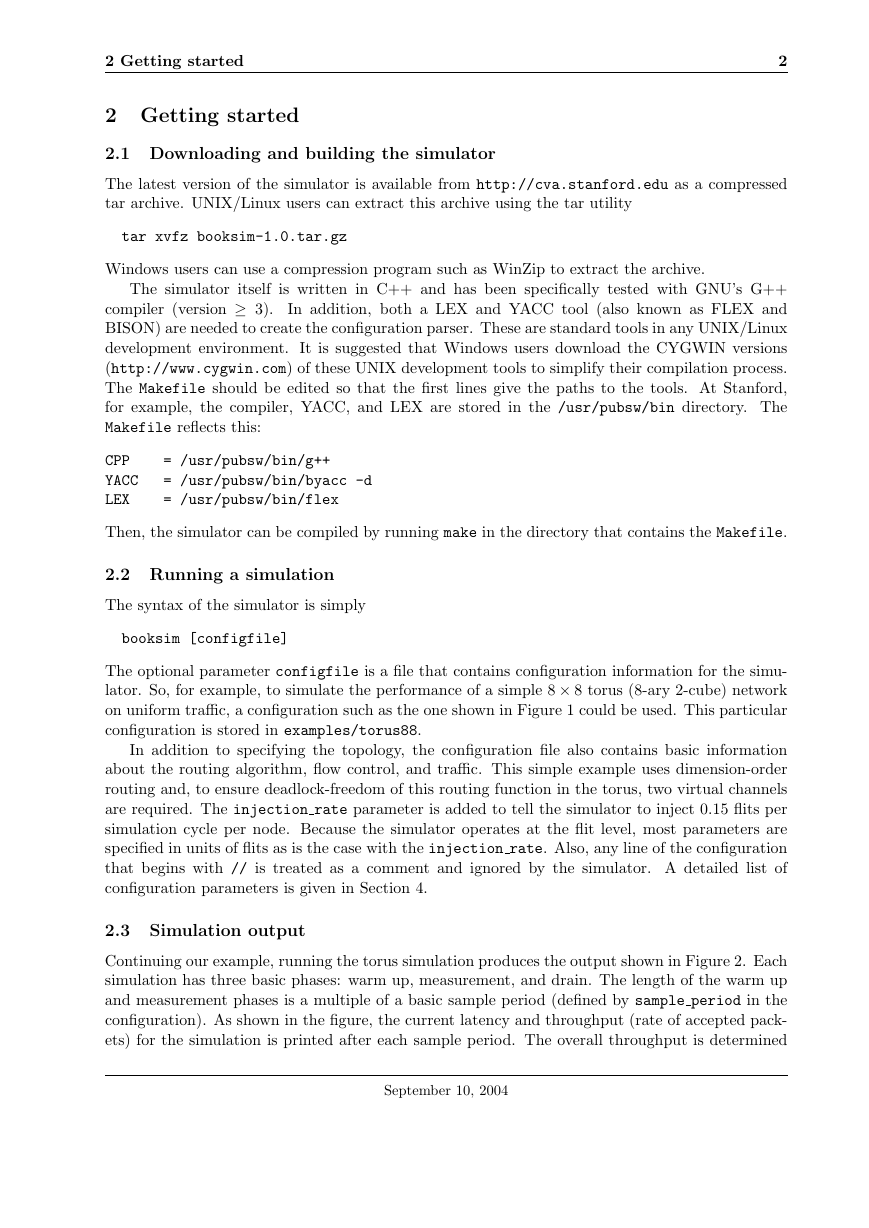2.2 Running a simulation The syntax of the simulator is simply booksim [configfile] The optional parameter configfile is a ﬁle that contains conﬁguration information for the simu- lator. So, for example, to simulate the performance of a simple 8 × 8 torus (8-ary 2-cube) network on uniform traﬃc, a conﬁguration such as the one shown in Figure 1 could be used. This particular conﬁguration is stored in examples/torus88. In addition to specifying the topology, the conﬁguration ﬁle also contains basic information about the routing algorithm, ﬂow control, and traﬃc. This simple example uses dimension-order routing and, to ensure deadlock-freedom of this routing function in the torus, two virtual channels are required. The injection rate parameter is added to tell the simulator to inject 0.15 ﬂits per simulation cycle per node. Because the simulator operates at the ﬂit level, most parameters are speciﬁed in units of ﬂits as is the case with the injection rate. Also, any line of the conﬁguration that begins with // is treated as a comment and ignored by the simulator. A detailed list of conﬁguration parameters is given in Section 4. 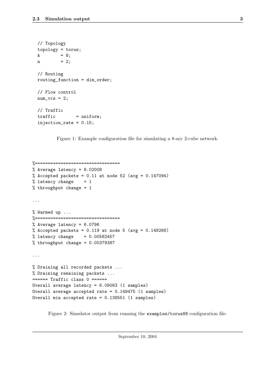2.3 Simulation output Continuing our example, running the torus simulation produces the output shown in Figure 2. Each simulation has three basic phases: warm up, measurement, and drain. The length of the warm up and measurement phases is a multiple of a basic sample period (deﬁned by sample period in the conﬁguration). As shown in the ﬁgure, the current latency and throughput (rate of accepted pack- ets) for the simulation is printed after each sample period. The overall throughput is determined September 10, 2004

2.3 Simulation output 3 // Topology topology = torus; k n = 8; = 2; // Routing routing_function = dim_order; // Flow control num_vcs = 2; // Traffic traffic injection_rate = 0.15; = uniform; Figure 1: Example conﬁguration ﬁle for simulating a 8-ary 2-cube network. %================================= % Average latency = 6.02008 % Accepted packets = 0.11 at node 52 (avg = 0.147094) % latency change = 1 % throughput change = 1 ... % Warmed up ... %================================= % Average latency = 6.0796 % Accepted packets = 0.119 at node 5 (avg = 0.148266) = 0.00562457 % latency change % throughput change = 0.00379387 ... % Draining all recorded packets ... % Draining remaining packets ... ====== Traffic class 0 ====== Overall average latency = 6.09083 (1 samples) Overall average accepted rate = 0.149475 (1 samples) Overall min accepted rate = 0.138551 (1 samples) Figure 2: Simulator output from running the examples/torus88 conﬁguration ﬁle. September 10, 2004

3 Examples 4 by the lowest throughput of all the destination in the network, but the average throughput is also displayed. After the warm up periods have passed, the simulator prints the “Warmed up” message and resets all the simulation statistics. Then, the measurement phase begins and statistics continue to be reported after each sample period. Once the measurement periods have passed, all the measurement packets are drained from the network before ﬁnal latency and throughput numbers are reported. Details of the conﬁguration parameters used to control the length of the simulation phases are covered in Section 4.7. 3 Examples One of the most basic performance measures of any interconnection network is its latency versus oﬀered load. Figure 3 shows a simple conﬁguration ﬁle for making this measurement in a 8-ary 2-mesh network under the transpose traﬃc pattern. This conﬁguration was used to generate Figure 25.2 in PPIN. The particular conﬁguration accounts for some small delays and pipelining of the input-queued router and also introduces a small input speedup to account for any ineﬃciencies in allocation. By running simulations for many increments of injection rate, the average latency curve can be found. Then, to compare the performance of dimension-order routing against several other routing algorithms, for example, the routing function option can be changed. 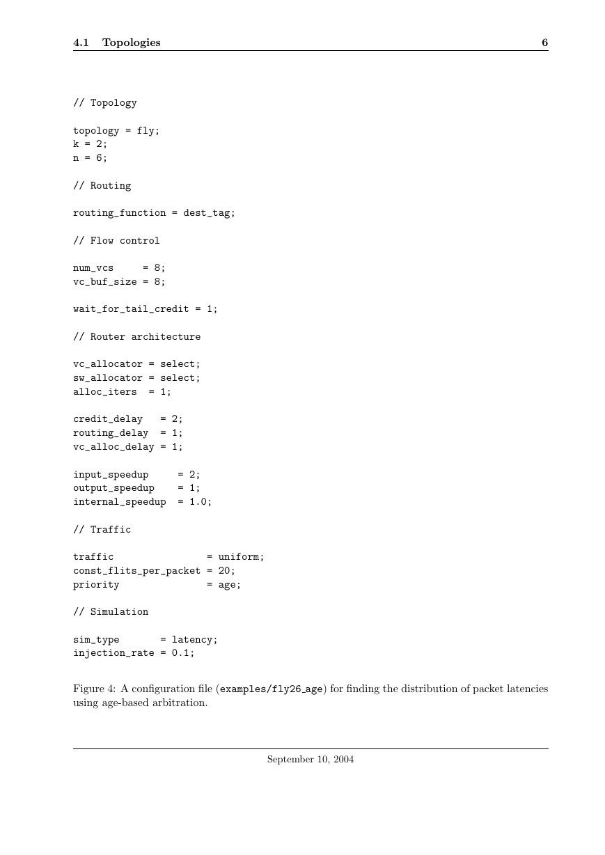Figure 4 shows a conﬁguration ﬁle that can be used to determine the distribution of packet latencies in a 2-ary 6-ﬂy network that uses age-based arbitration. Note the use of the priority conﬁguration parameter along with the select allocators that account for packet priorities. The simulator does not output latency distributions by default, but by editing trafficmanager.cpp, setting the conﬁguration variable DISPLAY LAT DIST to true, and recompiling, the distribution will be displayed at the end of the simulation. This technique was used to produced the distribution shown in Figure 25.12 of PPIN. As a ﬁnal example, Figure 5 shows the use of the special single-node topology to test the performance of a switch allocator — in this case, the iSLIP allocator. The in ports and out ports options set up a simulation of an 8 × 8 crossbar. 4 Conﬁguration parameters All information used to conﬁgure a simulation is passed through a conﬁguration ﬁle as illustrated by the example in Section 2.2. This section lists the existing conﬁguration parameters — a user can incorporate additional options by changing the booksim config.cpp ﬁle. 4.1 Topologies The topology parameter determines the underlying topology of the network and the simulator supports four basic topologies: fly mesh A k-ary n-ﬂy (butterﬂy) topology. The k parameter determines the network’s radix and the n parameter determines the network’s dimension. A k-ary n-mesh (mesh) topology. The k parameter determines the network’s radix and the n parameter determines the network’s dimension. September 10, 2004

4.1 Topologies 5 // Topology topology = mesh; k = 8; n = 2; // Routing routing_function = dim_order; // Flow control num_vcs = 8; vc_buf_size = 8; wait_for_tail_credit = 1; // Router architecture vc_allocator = islip; sw_allocator = islip; alloc_iters = 1; credit_delay = 2; routing_delay = 1; vc_alloc_delay = 1; input_speedup output_speedup internal_speedup = 1.0; = 2; = 1; // Traffic traffic const_flits_per_packet = 20; = transpose; // Simulation sim_type injection_rate = 0.1; = latency; Figure 3: A typical conﬁguration ﬁle (examples/mesh88 lat) for creating a latency versus oﬀered load curve for a 8-ary 2-mesh network. September 10, 2004

6 4.1 Topologies // Topology topology = fly; k = 2; n = 6; // Routing routing_function = dest_tag; // Flow control num_vcs = 8; vc_buf_size = 8; wait_for_tail_credit = 1; // Router architecture vc_allocator = select; sw_allocator = select; alloc_iters = 1; = 2; credit_delay = 1; routing_delay vc_alloc_delay = 1; input_speedup output_speedup internal_speedup = 1.0; = 2; = 1; // Traffic traffic const_flits_per_packet = 20; priority = age; = uniform; // Simulation sim_type injection_rate = 0.1; = latency; Figure 4: A conﬁguration ﬁle (examples/fly26 age) for ﬁnding the distribution of packet latencies using age-based arbitration. September 10, 2004

4.1 Topologies 7 // Topology = single; topology in_ports = 8; out_ports = 8; // Routing routing_function = single; // Flow control vc_allocator = islip; sw_allocator = islip; alloc_iters = 2; num_vcs vc_buf_size = 1000; = 8; wait_for_tail_credit = 0; // Simulation sim_type injection_rate = 0.1; = latency; Figure 5: A single-node conﬁguration ﬁle (examples/single) for testing the performance of a switch allocator. September 10, 2004

4.2 Routing algorithms 8 single A network with a single node, used for testing single router performance. The number of input and output ports for the node is determined by the in ports and out ports parameters, respectively. torus A k-ary n-cube (torus) topology. The k parameter determines the network’s radix and the n parameter determines the network’s dimension. Both the mesh and torus topologies support the addition of random link failures with the link failures parameter. The value of link failures determines the number of channels that are randomly removed from the topology and are thus no longer available for forwarding packets. Moreover, the randomization for failed channels is controlled by selecting an integer value for the fail seed parameter — a ﬁxed seed gives a ﬁxed set of failed channels, independent of other randomization in the simulation. Also, note that only certain routing functions support this feature (see Section 4.2). 4.2 Routing algorithms The routing function parameter selects a routing algorithm for the topology. Many routing algorithms need multiple virtual channels for deadlock freedom (VCDF). dim order Dimension-order routing. Works for the mesh topology (1 VCDF) and for the torus topology (2 VCDF). dim order bal Dimension-order routing for the torus topology with a more balanced use of VCs to avoid deadlock (2 VCDF). dim order ni A non-interfering version of dimension-order routing. Works on the torus or mesh topology and requires one VC per network terminal. min adapt A minimal adaptive routing algorithm for the mesh topology (2 VCDF) and for the torus topology (3 VCDF). planar adapt Planar-adaptive routing for the mesh topology (2 VCDF). Supports routing around failed channels. romm romm ni single valiant ROMM routing for the mesh (2 VCDF). Load is balanced by routing in two phases: one from the source to a random intermediate node in the minimal quadrant and a second from the intermediate to the destination. A non-interfering version of ROMM routing for the mesh that requires one VC per network terminal. A dummy routing function used for the single topology. Valiant’s randomized routing algorithm for the mesh (2 VCDF) and torus (4 VCDF) topology. valiant ni A non-interfering version of Valiant’s algorithm for the torus that requires 4 VCs per network terminal. Also, the simulator code is structured so that additional routing algorithms can be added with minimal changes to the overall simulator (see the routefunc.cpp ﬁle in the simulator’s source code). September 10, 2004

资料库

BookSim 2.0 User's Guide.pdf

相关推荐

网络技术

热门标签

最新资料