Journal of Machine Learning Research 15 (2014) 3133-3181
Submitted 11/13; Revised 4/14; Published 10/14
Do we Need Hundreds of Classifiers to Solve Real World
Classification Problems?
Manuel Fern´andez-Delgado
Eva Cernadas
Sen´en Barro
CITIUS: Centro de Investigaci´on en Tecnolox´ıas da Informaci´on da USC
University of Santiago de Compostela
Campus Vida, 15872, Santiago de Compostela, Spain
manuel.fernandez.delgado@usc.es
eva.cernadas@usc.es
senen.barro@usc.es
Dinani Amorim
Departamento de Tecnologia e Ciˆencias Sociais- DTCS
Universidade do Estado da Bahia
Av. Edgard Chastinet S/N - S˜ao Geraldo - Juazeiro-BA, CEP: 48.305-680, Brasil
dinaniamorim@gmail.com
Editor: Russ Greiner
Abstract
We evaluate 179 classifiers arising from 17 families (discriminant analysis, Bayesian,
neural networks, support vector machines, decision trees, rule-based classifiers, boosting,
bagging, stacking, random forests and other ensembles, generalized linear models, nearest-
neighbors, partial least squares and principal component regression, logistic and multino-
mial regression, multiple adaptive regression splines and other methods), implemented in
Weka, R (with and without the caret package), C and Matlab, including all the relevant
classifiers available today. We use 121 data sets, which represent the whole UCI data
base (excluding the large-scale problems) and other own real problems, in order to achieve
significant conclusions about the classifier behavior, not dependent on the data set col-
lection. The classifiers most likely to be the bests are the random forest (RF)
versions, the best of which (implemented in R and accessed via caret) achieves 94.1% of
the maximum accuracy overcoming 90% in the 84.3% of the data sets. However, the dif-
ference is not statistically significant with the second best, the SVM with Gaussian kernel
implemented in C using LibSVM, which achieves 92.3% of the maximum accuracy. A few
models are clearly better than the remaining ones: random forest, SVM with Gaussian
and polynomial kernels, extreme learning machine with Gaussian kernel, C5.0 and avNNet
(a committee of multi-layer perceptrons implemented in R with the caret package). The
random forest is clearly the best family of classifiers (3 out of 5 bests classifiers are RF),
followed by SVM (4 classifiers in the top-10), neural networks and boosting ensembles (5
and 3 members in the top-20, respectively).
Keywords: classification, UCI data base, random forest, support vector machine, neural
networks, decision trees, ensembles, rule-based classifiers, discriminant analysis, Bayesian
classifiers, generalized linear models, partial least squares and principal component re-
gression, multiple adaptive regression splines, nearest-neighbors, logistic and multinomial
regression
c2014 Manuel Fern´andez-Delgado, Eva Cernadas, Sen´en Barro and Dinani Amorim.
�
Fern´andez-Delgado, Cernadas, Barro and Amorim
1. Introduction
When a researcher or data analyzer faces to the classification of a data set, he/she usually
applies the classifier which he/she expects to be “the best one”. This expectation is condi-
tioned by the (often partial) researcher knowledge about the available classifiers. One reason
is that they arise from different fields within computer science and mathematics, i.e., they
belong to different “classifier families”. For example, some classifiers (linear discriminant
analysis or generalized linear models) come from statistics, while others come from symbolic
artificial intelligence and data mining (rule-based classifiers or decision-trees), some others
are connectionist approaches (neural networks), and others are ensembles, use regression or
clustering approaches, etc. A researcher may not be able to use classifiers arising from areas
in which he/she is not an expert (for example, to develop parameter tuning), being often
limited to use the methods within his/her domain of expertise. However, there is no certainty
that they work better, for a given data set, than other classifiers, which seem more “exotic”
to him/her. The lack of available implementation for many classifiers is a major drawback,
although it has been partially reduced due to the large amount of classifiers implemented
in R1 (mainly from Statistics), Weka2 (from the data mining field) and, in a lesser extend,
in Matlab using the Neural Network Toolbox3. Besides, the R package caret (Kuhn, 2008)
provides a very easy interface for the execution of many classifiers, allowing automatic pa-
rameter tuning and reducing the requirements on the researcher’s knowledge (about the
tunable parameter values, among other issues). Of course, the researcher can review the
literature to know about classifiers in families outside his/her domain of expertise and, if
they work better, to use them instead of his/her preferred classifier. However, usually the
papers which propose a new classifier compare it only to classifiers within the same family,
excluding families outside the author’s area of expertise. Thus, the researcher does not know
whether these classifiers work better or not than the ones that he/she already knows. On the
other hand, these comparisons are usually developed over a few, although expectedly rele-
vant, data sets. Given that all the classifiers (even the “good” ones) show strong variations
in their results among data sets, the average accuracy (over all the data sets) might be of
limited significance if a reduced collection of data sets is used (Maci`a and Bernad´o-Mansilla,
2014). Specifically, some classifiers with a good average performance over a reduced data
set collection could achieve significantly worse results when the collection is extended, and
conversely classifiers with sub-optimal performance on the reduced data collection could be
not so bad when more data sets are included. There are useful guidelines (Hothorn et al.,
2005; Eugster et al., 2014) to analyze and design benchmark exploratory and inferential
experiments, giving also a very useful framework to inspect the relationship between data
sets and classifiers.
Each time we find a new classifier or family of classifiers from areas outside our domain
of expertise, we ask ourselves whether that classifier will work better than the ones that we
use routinely. In order to have a clear idea of the capabilities of each classifier and family, it
would be useful to develop a comparison of a high number of classifiers arising from many
different families and areas of knowledge over a large collection of data sets. The objective
1. See http://www.r-project.org.
2. See http://www.cs.waikato.ac.nz/ml/weka.
3. See http://www.mathworks.es/products/neural-network.
3134
�
Do we Need Hundreds of Classifiers to Solve Real World Classification Problems?
is to select the classifier which more probably achieves the best performance for any data
set.
In the current paper we use a large collection of classifiers with publicly available
implementations (in order to allow future comparisons), arising from a wide variety of
classifier families, in order to achieve significant conclusions not conditioned by the number
and variety of the classifiers considered. Using a high number of classifiers it is probable that
some of them will achieve the “highest” possible performance for each data set, which can
be used as reference (maximum accuracy) to evaluate the remaining classifiers. However,
according to the No-Free-Lunch theorem (Wolpert, 1996), the best classifier will not be the
same for all the data sets. Using classifiers from many families, we are not restricting the
significance of our comparison to one specific family among many available methods. Using
a high number of data sets, it is probable that each classifier will work well in some data
sets and not so well in others, increasing the evaluation significance. Finally, considering
the availability of several alternative implementations for the most popular classifiers, their
comparison may also be interesting. The current work pursues: 1) to select the globally
best classifier for the selected data set collection; 2) to rank each classifier and family
according to its accuracy; 3) to determine, for each classifier, its probability of achieving
the best accuracy, and the difference between its accuracy and the best one; 4) to evaluate
the classifier behavior varying the data set properties (complexity, #patterns, #classes and
#inputs).
Some recent papers have analyzed the comparison of classifiers over large collection of
data sets. OpenML (Vanschoren et al., 2012), is a complete web interface4 to anonymously
access an experiment data base including 86 data sets from the UCI machine learning data
base (Bache and Lichman, 2013) and 93 classifiers implemented in Weka. Although plug-
ins for R, Knime and RapidMiner are under development, currently it only allows to use
Weka classifiers. This environment allows to send queries about the classifier behavior with
respect to tunable parameters, considering several common performance measures, feature
selection techniques and bias-variance analysis. There is also an interesting analysis (Maci`a
and Bernad´o-Mansilla, 2014) about the use of the UCI repository launching several inter-
esting criticisms about the usual practice in experimental comparisons. In the following,
we synthesize these criticisms (the italicized sentences are literal cites) and describe how we
tried to avoid them in our paper:
1. The criterion used to select the data set collection (which is usually reduced) may
bias the comparison results. The same authors stated (Maci`a et al., 2013) that the
superiority of a classifier may be restricted to a given domain characterized by some
complexity measures, studying why and how the data set selection may change the
results of classifier comparisons. Following these suggestions, we use all the data sets
in the UCI classification repository, in order to avoid that a small data collection
invalidate the conclusions of the comparison. This paper also emphasizes that the
UCI repository was not designed to be a complete, reliable framework composed of
standardized real samples.
2. The issue about (1) whether the selection of learners is representative enough and (2)
whether the selected learners are properly configured to work at their best performance
4. See http://expdb.cs.kuleuven.be/expdb.
3135
�
Fern´andez-Delgado, Cernadas, Barro and Amorim
suggests that proposals of new classifiers usually design and tune them carefully, while
the reference classifiers are run using a baseline configuration. This issue is also related
to the lack of deep knowledge and experience about the details of all the classifiers with
available implementations, so that the researchers usually do not pay much attention
about the selected reference algorithms, which may consequently bias the results in
favour of the proposed algorithm. With respect to this criticism, in the current paper
we do not propose any new classifier nor changes on existing approaches, so we are not
interested in favour any specific classifier, although we are more experienced with some
classifier than others (for example, with respect to the tunable parameter values). We
develop in this work a parameter tuning in the majority of the classifiers used (see
below), selecting the best available configuration over a training set. Specifically, the
classifiers implemented in R using caret automatically tune these parameters and,
even more important, using pre-defined (and supposedly meaningful) values. This
fact should compensate our lack of experience about some classifiers, and reduce its
relevance on the results.
3. It is still impossible to determine the maximum attainable accuracy for a data set,
so that it is difficult to evaluate the true quality of each classifier. In our paper, we
use a large amount of classifiers (179) from many different families, so we hypothesize
that the maximum accuracy achieved by some classifier is the maximum attainable
accuracy for that data set:
i.e., we suppose that if no classifier in our collection is
able to reach higher accuracy, no one will reach. We can not test the validity of this
hypothesis, but it seems reasonable that, when the number of classifiers increases,
some of them will achieve the largest possible accuracy.
4. Since the data set complexity (measured somehow by the maximum attainable ac-
curacy) is unknown, we do not know if the classification error is caused by unfitted
classifier design (learner’s limitation) or by intrinsic difficulties of the problem (data
limitation). In our work, since we consider that the attainable accuracy is the maxi-
mum accuracy achieved by some classifier in our collection, we can consider that low
accuracies (with respect to this maximum accuracy) achieved by other classifiers are
always caused by classifier limitations.
5. The lack of standard data partitioning, defining training and testing data for cross-
validation trials. Simply the use of different data partitionings will eventually bias the
results, and make the comparison between experiments impossible, something which is
also emphasized by other researchers (Vanschoren et al., 2012). In the current paper,
each data set uses the same partitioning for all the classifiers, so that this issue can not
bias the results favouring any classifier. Besides, the partitions are publicly available
(see Section 2.1), in order to make possible the experiment replication.
The paper is organized as follows: the Section 2 describes the collection of data sets and
classifiers considered in this work; the Section 3 discusses the results of the experiments,
and the Section 4 compiles the conclusions of the research developed.
3136
�
Do we Need Hundreds of Classifiers to Solve Real World Classification Problems?
2. Materials and Methods
In the following paragraphs we describe the materials (data sets) and methods (classifiers)
used to develop this comparison.
Data set
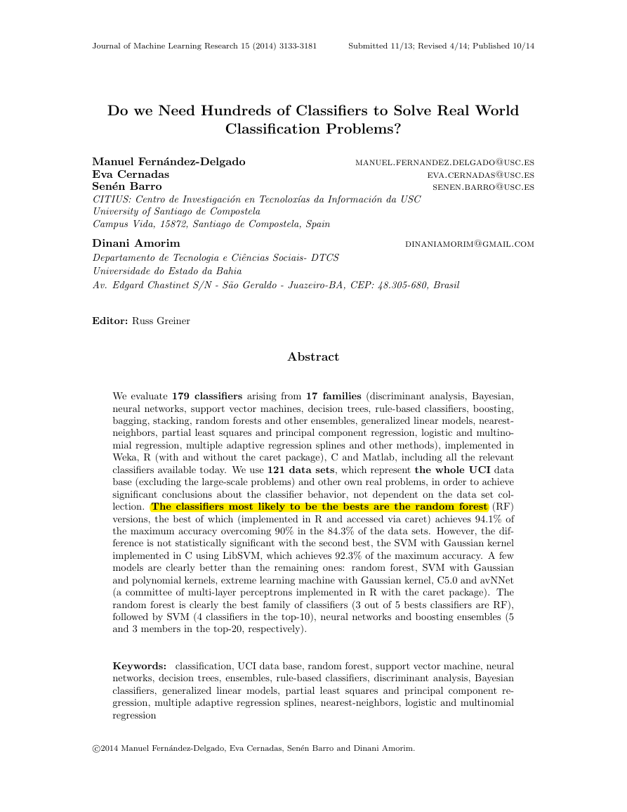
#pat. #inp. #cl. %Maj.
Data set
#pat. #inp. #cl. %Maj.
abalone
ac-inflam
acute-nephritis
adult
annealing
arrhythmia
audiology-std
balance-scale
balloons
bank
blood
breast-cancer
bc-wisc
bc-wisc-diag
bc-wisc-prog
breast-tissue
car
ctg-10classes
ctg-3classes
chess-krvk
chess-krvkp
congress-voting
conn-bench-sonar
conn-bench-vowel
connect-4
contrac
credit-approval
cylinder-bands
dermatology
echocardiogram
ecoli
4177
120
120
48842
798
452
226
625
16
45211
748
286
699
569
198
106
1728
2126
2126
28056
3196
435
208
528
67557
1473
690
512
366
131
336
8
6
6
14
38
262
59
4
4
17
4
9
9
30
33
9
6
21
21
6
36
16
60
11
42
9
15
35
34
10
7
3
2
2
2
6
13
18
3
2
2
2
2
2
2
2
6
4
10
3
18
2
2
2
11
2
3
2
2
6
2
8
flags
glass
haberman-survival
hayes-roth
ilpd-indian-liver
image-segmentation
energy-y1
energy-y2
fertility
heart-va
hepatitis
hill-valley
horse-colic
heart-cleveland
heart-hungarian
heart-switzerland
34.6
50.8
58.3
75.9
76.2
54.2
26.3
46.1
56.2
88.5
76.2
70.3
65.5
62.7
76.3
20.7
70.0
27.2
77.8
16.2
52.2
61.4
53.4
9.1
75.4
42.7
55.5
60.9
30.6 molec-biol-promoter
67.2
42.6
low-res-spect
lung-cancer
lymphography
mammographic
miniboone
lenses
letter
libras
ionosphere
iris
led-display
molec-biol-splice
monks-1
magic
768
768
100
194
214
306
132
303
294
123
200
155
606
300
583
210
351
150
1000
24
20000
360
531
32
148
19020
961
130064
106
3190
124
8
8
9
28
9
3
3
13
12
12
12
19
100
25
9
19
33
4
7
4
16
90
100
56
18
10
5
50
57
60
6
3
3
2
8
6
2
3
5
2
2
5
2
2
2
2
7
2
3
10
3
26
15
9
3
4
2
2
2
2
3
2
46.9
49.9
88.0
30.9
35.5
73.5
38.6
54.1
63.9
39.0
28.0
79.3
50.7
63.7
71.4
14.3
64.1
33.3
11.1
62.5
4.1
6.7
51.9
40.6
54.7
64.8
53.7
71.9
50.0
51.9
50.0
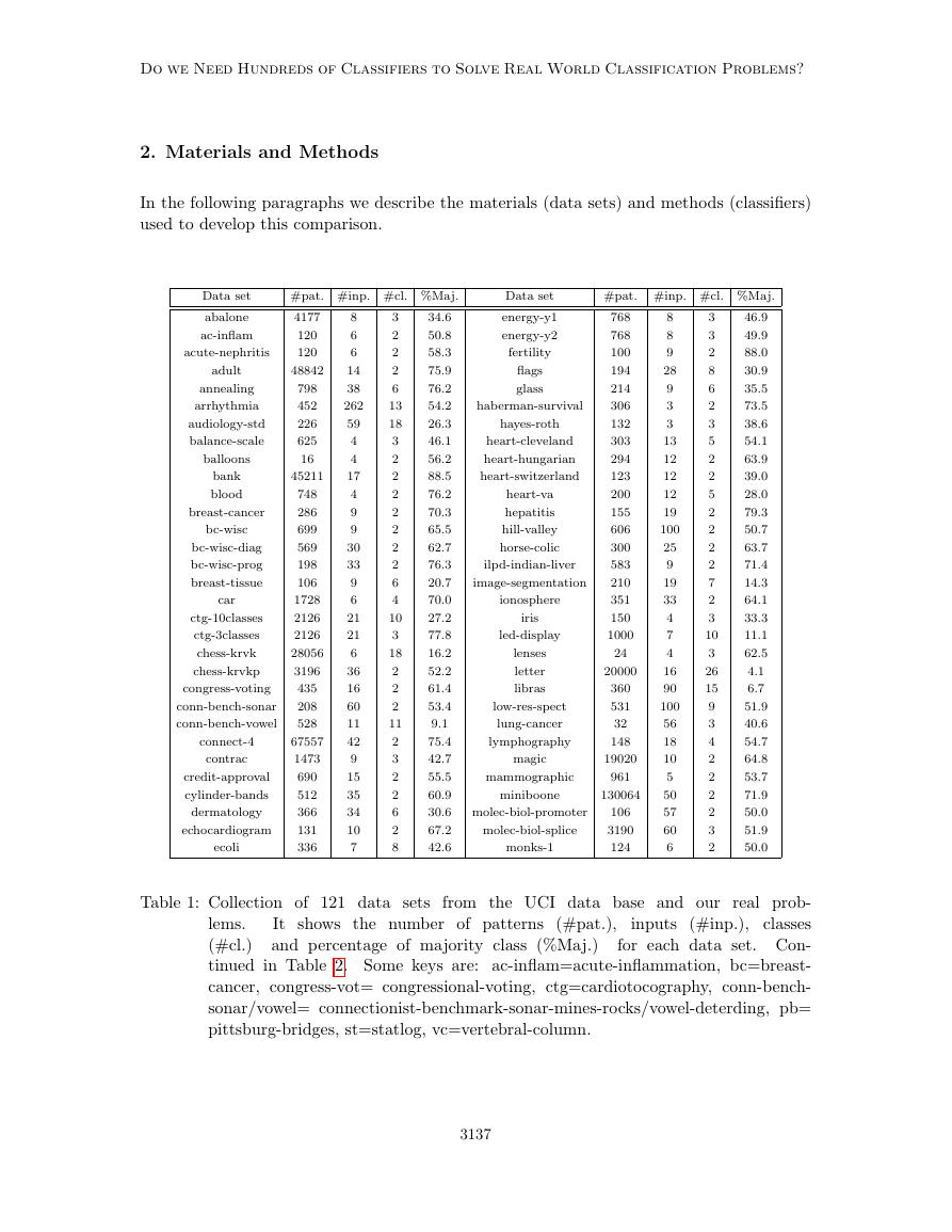
It shows the number of patterns (#pat.),
and percentage of majority class (%Maj.)
Table 1: Collection of 121 data sets from the UCI data base and our real prob-
inputs (#inp.), classes
lems.
(#cl.)
for each data set. Con-
tinued in Table 2. Some keys are: ac-inflam=acute-inflammation, bc=breast-
cancer, congress-vot= congressional-voting, ctg=cardiotocography, conn-bench-
sonar/vowel= connectionist-benchmark-sonar-mines-rocks/vowel-deterding, pb=
pittsburg-bridges, st=statlog, vc=vertebral-column.
3137
�
Fern´andez-Delgado, Cernadas, Barro and Amorim
2.1 Data Sets
We use the whole UCI machine learning repository, the most widely used data base in the
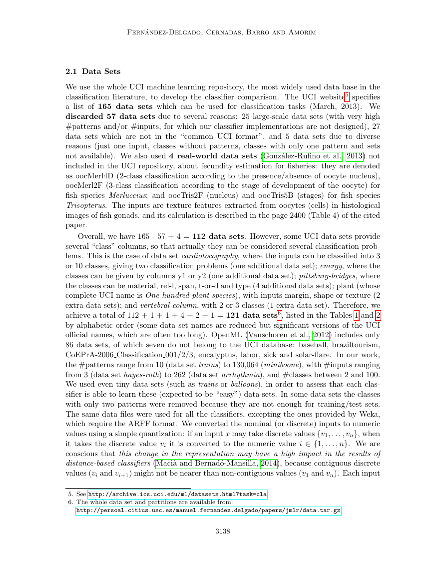
classification literature, to develop the classifier comparison. The UCI website5 specifies
a list of 165 data sets which can be used for classification tasks (March, 2013). We
discarded 57 data sets due to several reasons: 25 large-scale data sets (with very high
#patterns and/or #inputs, for which our classifier implementations are not designed), 27
data sets which are not in the “common UCI format”, and 5 data sets due to diverse
reasons (just one input, classes without patterns, classes with only one pattern and sets
not available). We also used 4 real-world data sets (Gonz´alez-Rufino et al., 2013) not
included in the UCI repository, about fecundity estimation for fisheries: they are denoted
as oocMerl4D (2-class classification according to the presence/absence of oocyte nucleus),
oocMerl2F (3-class classification according to the stage of development of the oocyte) for
fish species Merluccius; and oocTris2F (nucleus) and oocTris5B (stages) for fish species
Trisopterus. The inputs are texture features extracted from oocytes (cells) in histological
images of fish gonads, and its calculation is described in the page 2400 (Table 4) of the cited
paper.
Overall, we have 165 - 57 + 4 = 112 data sets. However, some UCI data sets provide
several “class” columns, so that actually they can be considered several classification prob-
lems. This is the case of data set cardiotocography, where the inputs can be classified into 3
or 10 classes, giving two classification problems (one additional data set); energy, where the
classes can be given by columns y1 or y2 (one additional data set); pittsburg-bridges, where
the classes can be material, rel-l, span, t-or-d and type (4 additional data sets); plant (whose
complete UCI name is One-hundred plant species), with inputs margin, shape or texture (2
extra data sets); and vertebral-column, with 2 or 3 classes (1 extra data set). Therefore, we
achieve a total of 112 + 1 + 1 + 4 + 2 + 1 = 121 data sets6, listed in the Tables 1 and 2
by alphabetic order (some data set names are reduced but significant versions of the UCI
official names, which are often too long). OpenML (Vanschoren et al., 2012) includes only
86 data sets, of which seven do not belong to the UCI database: baseball, braziltourism,
CoEPrA-2006 Classification 001/2/3, eucalyptus, labor, sick and solar-flare. In our work,
the #patterns range from 10 (data set trains) to 130,064 (miniboone), with #inputs ranging
from 3 (data set hayes-roth) to 262 (data set arrhythmia), and #classes between 2 and 100.
We used even tiny data sets (such as trains or balloons), in order to assess that each clas-
sifier is able to learn these (expected to be “easy”) data sets. In some data sets the classes
with only two patterns were removed because they are not enough for training/test sets.
The same data files were used for all the classifiers, excepting the ones provided by Weka,
which require the ARFF format. We converted the nominal (or discrete) inputs to numeric
values using a simple quantization: if an input x may take discrete values {v1, . . . , vn}, when
it takes the discrete value vi it is converted to the numeric value i ∈ {1, . . . , n}. We are
conscious that this change in the representation may have a high impact in the results of
distance-based classifiers (Maci`a and Bernad´o-Mansilla, 2014), because contiguous discrete
values (vi and vi+1) might not be nearer than non-contiguous values (v1 and vn). Each input
5. See http://archive.ics.uci.edu/ml/datasets.html?task=cla.
6. The whole data set and partitions are available from:
http://persoal.citius.usc.es/manuel.fernandez.delgado/papers/jmlr/data.tar.gz.
3138
�
Do we Need Hundreds of Classifiers to Solve Real World Classification Problems?
Data set
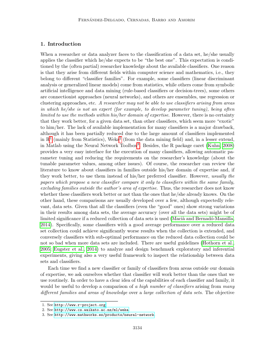
#pat. #inp. #cl. %Maj.
Data set
#pat. #inp. #cl. %Maj.
monks-2
monks-3
mushroom
musk-1
musk-2
nursery
oocMerl2F
oocMerl4D
oocTris2F
oocTris5B
optical
ozone
page-blocks
parkinsons
pendigits
pima
pb-MATERIAL
pb-REL-L
pb-SPAN
pb-T-OR-D
pb-TYPE
planning
plant-margin
plant-shape
plant-texture
post-operative
primary-tumor
ringnorm
seeds
semeion
169
3190
8124
476
6598
12960
1022
1022
912
912
3823
2536
5473
195
7494
768
106
103
92
102
105
182
1600
1600
1600
90
330
7400
210
1593
6
6
21
166
166
8
25
41
25
32
62
72
10
22
16
8
4
4
4
4
4
12
64
64
64
8
17
20
7
256
2
2
2
2
2
5
3
2
2
3
10
2
5
2
10
2
3
3
3
2
6
2
100
100
100
3
15
2
3
10
62.1
50.8
51.8
56.5
84.6
33.3
67.0
68.7
57.8
57.6
10.2
97.1
89.8
75.4
10.4
65.1
74.5
51.5
52.2
86.3
41.9
71.4
1.0
1.0
1.0
71.1
25.4
50.5
33.3
10.2
soybean
spambase
spect
spectf
st-australian-credit
st-german-credit
st-heart
st-image
st-landsat
st-shuttle
st-vehicle
steel-plates
synthetic-control
teaching
thyroid
tic-tac-toe
titanic
trains
twonorm
vc-2classes
vc-3classes
wall-following
waveform
waveform-noise
wine
wine-quality-red
wine-quality-white
yeast
zoo
307
4601
80
80
690
1000
270
2310
4435
43500
846
1941
600
151
3772
958
2201
10
7400
310
310
5456
5000
5000
179
1599
4898
1484
101
35
57
22
44
14
24
13
18
36
9
18
27
60
5
21
9
3
28
20
6
6
24
21
40
13
11
11
8
16
18
2
2
2
2
2
2
7
6
7
4
7
6
3
3
2
2
2
2
2
3
4
3
3
3
6
7
10
7
13.0
60.6
67.1
50.0
67.8
70.0
55.6
14.3
24.2
78.4
25.8
34.7
16.7
34.4
92.5
65.3
67.7
50.0
50.0
67.7
48.4
40.4
33.9
33.8
39.9
42.6
44.9
31.2
40.6
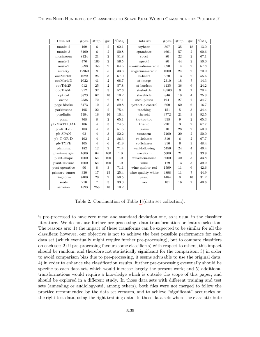
Table 2: Continuation of Table 1 (data set collection).
is pre-processed to have zero mean and standard deviation one, as is usual in the classifier
literature. We do not use further pre-processing, data transformation or feature selection.
The reasons are: 1) the impact of these transforms can be expected to be similar for all the
classifiers; however, our objective is not to achieve the best possible performance for each
data set (which eventually might require further pre-processing), but to compare classifiers
on each set; 2) if pre-processing favours some classifier(s) with respect to others, this impact
should be random, and therefore not statistically significant for the comparison; 3) in order
to avoid comparison bias due to pre-processing, it seems advisable to use the original data;
4) in order to enhance the classification results, further pre-processing eventually should be
specific to each data set, which would increase largely the present work; and 5) additional
transformations would require a knowledge which is outside the scope of this paper, and
should be explored in a different study. In those data sets with different training and test
sets (annealing or audiology-std, among others), both files were not merged to follow the
practice recommended by the data set creators, and to achieve “significant” accuracies on
the right test data, using the right training data. In those data sets where the class attribute
3139
�
Fern´andez-Delgado, Cernadas, Barro and Amorim
must be defined grouping several values (in data set abalone) we follow the instructions in
the data set description (file data.names). Given that our classifiers are not oriented to
data with missing features, the missing inputs are treated as zero, which should not bias the
comparison results. For each data set (abalone) two data files are created: abalone R.dat,
designed to be read by the R, C and Matlab classifiers, and abalone.arff, designed to be
read by the Weka classifiers.
2.2 Classifiers
We use 179 classifiers implemented in C/C++, Matlab, R and Weka. Excepting the
Matlab classifiers, all of them are free software. We only developed own versions in C for
the classifiers proposed by us (see below). Some of the R programs use directly the package
that provides the classifier, but others use the classifier through the interface train provided
by the caret7 package. This function develops the parameter tuning, selecting the values
which maximize the accuracy according to the validation selected (leave-one-out, k-fold,
etc.). The caret package also allows to define the number of values used for each tunable
parameter, although the specific values can not be selected. We used all the classifiers
provided by Weka, running the command-line version of the java class for each classifier.
OpenML uses 93 Weka classifiers, from which we included 84. We could not include
in our collection the remaining 9 classifiers: ADTree, alternating decision tree (Freund
and Mason, 1999); AODE, aggregating one-dependence estimators (Webb et al., 2005);
Id3 (Quinlan, 1986); LBR, lazy Bayesian rules (Zheng and Webb, 2000); M5Rules (Holmes
et al., 1999); Prism (Cendrowska, 1987); ThresholdSelector; VotedPerceptron (Freund and
Schapire, 1998) and Winnow (Littlestone, 1988). The reason is that they only accept
nominal (not numerical) inputs, while we converted all the inputs to numeric values. Be-
sides, we did not use classifiers ThresholdSelector, VotedPerceptron and Winnow, included
in openML, because they accept only two-class problems. Note that classifiers Locally-
WeightedLearning and RippleDownRuleLearner (Vanschoren et al., 2012) are included in
our collection as LWL and Ridor respectively. Furthermore, we also included other 36 clas-
sifiers implemented in R, 48 classifiers in R using the caret package, as well as 6 classifiers
implemented in C and other 5 in Matlab, summing up to 179 classifiers.
In the following, we briefly describe the 179 classifiers of the different families identi-
fied by acronyms (DA, BY, etc., see below), their names and implementations, coded as
name implementation, where implementation can be C, m (Matlab), R, t (in R using
caret) and w (Weka), and their tunable parameter values (the notation A:B:C means from
A to C step B). We found errors using several classifiers accessed via caret, but we used
the corresponding R packages directly. This is the case of lvq, bdk, gaussprLinear, glm-
net, kernelpls, widekernelpls, simpls, obliqueTree, spls, gpls, mars, multinom, lssvmRadial,
partDSA, PenalizedLDA, qda, QdaCov, mda, rda, rpart, rrlda, sddaLDA, sddaQDA and
sparseLDA. Some other classifiers as Linda, smda and xyf (not listed below) gave errors
(both with and without caret) and could not be included in this work. In the R and caret
implementations, we specify the function and, in typewriter font, the package which provide
that classifier (the function name is absent when it is is equal to the classifier).
7. See http://caret.r-forge.r-project.org.
3140
�


 2023年江西萍乡中考道德与法治真题及答案.doc
 2012年重庆南川中考生物真题及答案.doc
 2013年江西师范大学地理学综合及文艺理论基础考研真题.doc
 2020年四川甘孜小升初语文真题及答案I卷.doc
 2020年注册岩土工程师专业基础考试真题及答案.doc
 2023-2024学年福建省厦门市九年级上学期数学月考试题及答案.doc
 2021-2022学年辽宁省沈阳市大东区九年级上学期语文期末试题及答案.doc
 2022-2023学年北京东城区初三第一学期物理期末试卷及答案.doc
 2018上半年江西教师资格初中地理学科知识与教学能力真题及答案.doc
 2012年河北国家公务员申论考试真题及答案-省级.doc
 2020-2021学年江苏省扬州市江都区邵樊片九年级上学期数学第一次质量检测试题及答案.doc
 2022下半年黑龙江教师资格证中学综合素质真题及答案.doc