LONG SHORT-TERM MEMORY
Neural Computation (�):����{����, � �
Sepp Hochreiter
Jurgen Schmidhuber
Fakultat fur Informatik
IDSIA
Technische Universitat Munchen
Corso Elvezia ��
��� � Munchen, Germany
� �� Lugano, Switzerland
hochreit@informatik.tu-muenchen.de
juergen@idsia.ch
http://www�.informatik.tu-muenchen.de/~hochreit
http://www.idsia.ch/~juergen
Abstract
Learning to store information over extended time intervals via recurrent backpropagation
takes a very long time, mostly due to insucient, decaying error back ow. We briey review
Hochreiter's � � analysis of this problem, then address it by introducing a novel, ecient,
gradient-based method called \Long Short-Term Memory" (LSTM). Truncating the gradient
where this does not do harm, LSTM can learn to bridge minimal time lags in excess of ����
discrete time steps by enforcing constant error ow through \constant error carrousels" within
special units. Multiplicative gate units learn to open and close access to the constant error
ow. LSTM is local in space and time; its computational complexity per time step and weight
is O(�). Our experiments with articial data involve local, distributed, real-valued, and noisy
pattern representations. In comparisons with RTRL, BPTT, Recurrent Cascade-Correlation,
Elman nets, and Neural Sequence Chunking, LSTM leads to many more successful runs, and
learns much faster. LSTM also solves complex, articial long time lag tasks that have never
been solved by previous recurrent network algorithms.
�
INTRODUCTION
Recurrent networks can in principle use their feedback connections to store representations of
recent input events in form of activations (\short-term memory", as opposed to \long-term mem-
ory" embodied by slowly changing weights). This is potentially signicant for many applications,
including speech processing, non-Markovian control, and music composition (e.g., Mozer � �).
The most widely used algorithms for learning what to put in short-term memory, however, take
too much time or do not work well at all, especially when minimal time lags between inputs and
corresponding teacher signals are long. Although theoretically fascinating, existing methods do
not provide clear practical advantages over, say, backprop in feedforward nets with limited time
windows. This paper will review an analysis of the problem and suggest a remedy.
The problem. With conventional \Back-Propagation Through Time" (BPTT, e.g., Williams
and Zipser � �, Werbos � ��) or \Real-Time Recurrent Learning" (RTRL, e.g., Robinson and
Fallside � ��), error signals \owing backwards in time" tend to either (�) blow up or (�) vanish:
the temporal evolution of the backpropagated error exponentially depends on the size of the
weights (Hochreiter � �). Case (�) may lead to oscillating weights, while in case (�) learning to
bridge long time lags takes a prohibitive amount of time, or does not work at all (see section �).
The remedy. This paper presents \Long Short-Term Memory" (LSTM), a novel recurrent
network architecture in conjunction with an appropriate gradient-based learning algorithm. LSTM
is designed to overcome these error back-ow problems. It can learn to bridge time intervals in
excess of ���� steps even in case of noisy, incompressible input sequences, without loss of short
time lag capabilities. This is achieved by an ecient, gradient-based algorithm for an architecture
�
�
enforcing constant (thus neither exploding nor vanishing) error ow through internal states of
special units (provided the gradient computation is truncated at certain architecture-specic points
| this does not aect long-term error ow though).
Outline of paper. Section � will briey review previous work. Section � begins with an outline
of the detailed analysis of vanishing errors due to Hochreiter (� �). It will then introduce a naive
approach to constant error backprop for didactic purposes, and highlight its problems concerning
information storage and retrieval. These problems will lead to the LSTM architecture as described
in Section �. Section � will present numerous experiments and comparisons with competing
methods. LSTM outperforms them, and also learns to solve complex, articial tasks no other
recurrent net algorithm has solved. Section � will discuss LSTM's limitations and advantages. The
appendix contains a detailed description of the algorithm (A.�), and explicit error ow formulae
(A.�).
� PREVIOUS WORK
This section will focus on recurrent nets with time-varying inputs (as opposed to nets with sta-
tionary inputs and xpoint-based gradient calculations, e.g., Almeida � ��, Pineda � ��).
Gradient-descent variants. The approaches of Elman (� ��), Fahlman (� �), Williams
(� � ), Schmidhuber (� �a), Pearlmutter (� � ), and many of the related algorithms in Pearl-
mutter's comprehensive overview (� �) suer from the same problems as BPTT and RTRL (see
Sections � and �).
Time-delays. Other methods that seem practical for short time lags only are Time-Delay
Neural Networks (Lang et al. � �) and Plate's method (Plate � �), which updates unit activa-
tions based on a weighted sum of old activations (see also de Vries and Principe � �). Lin et al.
(� �) propose variants of time-delay networks called NARX networks.
Time constants. To deal with long time lags, Mozer (� �) uses time constants inuencing
changes of unit activations (deVries and Principe's above-mentioned approach (� �) may in fact
be viewed as a mixture of TDNN and time constants). For long time lags, however, the time
constants need external ne tuning (Mozer � �). Sun et al.'s alternative approach (� �) updates
the activation of a recurrent unit by adding the old activation and the (scaled) current net input.
The net input, however, tends to perturb the stored information, which makes long-term storage
impractical.
Ring's approach. Ring (� �) also proposed a method for bridging long time lags. Whenever
a unit in his network receives conicting error signals, he adds a higher order unit inuencing
appropriate connections. Although his approach can sometimes be extremely fast, to bridge a
time lag involving ��� steps may require the addition of ��� units. Also, Ring's net does not
generalize to unseen lag durations.
Bengio et al.'s approaches. Bengio et al. (� �) investigate methods such as simulated
annealing, multi-grid random search, time-weighted pseudo-Newton optimization, and discrete
error propagation. Their \latch" and \�-sequence" problems are very similar to problem �a with
minimal time lag ��� (see Experiment �). Bengio and Frasconi (� �) also propose an EM approach
for propagating targets. With n so-called \state networks", at a given time, their system can be
in one of only n dierent states. See also beginning of Section �. But to solve continuous problems
such as the \adding problem" (Section �.�), their system would require an unacceptable number
of states (i.e., state networks).
Kalman lters. Puskorius and Feldkamp (� �) use Kalman lter techniques to improve
recurrent net performance. Since they use \a derivative discount factor imposed to decay expo-
nentially the eects of past dynamic derivatives," there is no reason to believe that their Kalman
Filter Trained Recurrent Networks will be useful for very long minimal time lags.
Second order nets. We will see that LSTM uses multiplicative units (MUs) to protect error
ow from unwanted perturbations. It is not the rst recurrent net method using MUs though.
For instance, Watrous and Kuhn (� �) use MUs in second order nets. Some dierences to LSTM
are: (�) Watrous and Kuhn's architecture does not enforce constant error ow and is not designed
�
�
to solve long time lag problems. (�) It has fully connected second-order sigma-pi units, while the
LSTM architecture's MUs are used only to gate access to constant error ow. (�) Watrous and
Kuhn's algorithm costs O(W
) operations per time step, ours only O(W ), where W is the number
�
of weights. See also Miller and Giles (� �) for additional work on MUs.
Simple weight guessing. To avoid long time lag problems of gradient-based approaches we
may simply randomly initialize all network weights until the resulting net happens to classify all
training sequences correctly. In fact, recently we discovered (Schmidhuber and Hochreiter � �,
Hochreiter and Schmidhuber � �, � �) that simple weight guessing solves many of the problems
in (Bengio � �, Bengio and Frasconi � �, Miller and Giles � �, Lin et al. � �) faster than
the algorithms proposed therein. This does not mean that weight guessing is a good algorithm.
It just means that the problems are very simple. More realistic tasks require either many free
parameters (e.g., input weights) or high weight precision (e.g., for continuous-valued parameters),
such that guessing becomes completely infeasible.
Adaptive sequence chunkers. Schmidhuber's hierarchical chunker systems (� �b, � �)
do have a capability to bridge arbitrary time lags, but only if there is local predictability across the
subsequences causing the time lags (see also Mozer � �). For instance, in his postdoctoral thesis
(� �), Schmidhuber uses hierarchical recurrent nets to rapidly solve certain grammar learning
tasks involving minimal time lags in excess of ���� steps. The performance of chunker systems,
however, deteriorates as the noise level increases and the input sequences become less compressible.
LSTM does not suer from this problem.
� CONSTANT ERROR BACKPROP
�.� EXPONENTIALLY DECAYING ERROR
Conventional BPTT (e.g. Williams and Zipser � �). Output unit k 's target at time t is
denoted by d
(t). Using mean squared error, k 's error signal is
k
#
(t) = f
(net
(t))(d
(t) y
(t));
k
k
k
k
�
k
where
i
y
(t) = f
(net
(t))
i
i
is the activation of a non-input unit i with dierentiable activation function f
,
i
X
j
net
(t) =
w
y
(t �)
i
ij
j
is unit i's current net input, and w
is the weight on the connection from unit j to i. Some
ij
non-output unit j 's backpropagated error signal is
�
X
#
(t) = f
(net
(t))
w
#
(t + �):
j
j
ij
i
j
i
The corresponding contribution to w
's total weight update is #
(t)y
(t �), where is the
j l
j
l
learning rate, and l stands for an arbitrary unit connected to unit j .
Outline of Hochreiter's analysis (� �, page � -��). Suppose we have a fully connected
net whose non-input unit indices range from � to n. Let us focus on local error ow from unit u
to unit v (later we will see that the analysis immediately extends to global error ow). The error
occurring at an arbitrary unit u at time step t is propagated \back into time" for q time steps, to
an arbitrary unit v . This will scale the error by the following factor:
(
�
@ #
(t q)
v
uv
v
v
f
(net
(t �))w
q = �
=
:
(�)
P
�
l
n
@ #
(tq+�)
@ #
(t)
u
v
v
lv
f
(net
(t q))
w
q > �
l=�
@ #
(t)
u
�
�
With l
= v and l
= u, we obtain:
q
�
@ #
(t q)
v
�
n
n
q
X
X
Y
=
: : :
f
(net
(t m))w
(�)
l
m
l
l
l
m
m
m�
@ #
(t)
u
l
=�
l
=�
m=�
�
q�
(proof by induction). The sum of the n
terms
f
(net
(t m))w
determines the
m=�
l
m
l
l
l
m
m
m�
q�
�
Q
q
total error back ow (note that since the summation terms may have dierent signs, increasing
the number of units n does not necessarily increase error ow).
Intuitive explanation of equation (�). If
�
jf
(net
(t m))w
j > �:�
l
m
l
l
l
m
m
m�
for all m (as can happen, e.g., with linear f
) then the largest product increases exponentially
l
m
with q . That is, the error blows up, and conicting error signals arriving at unit v can lead to
oscillating weights and unstable learning (for error blow-ups or bifurcations see also Pineda � ��,
Baldi and Pineda � �, Doya � �). On the other hand, if
�
jf
(net
(t m))w
j < �:�
l
m
l
l
l
m
m
m�
for all m, then the largest product decreases exponentially with q . That is, the error vanishes, and
nothing can be learned in acceptable time.
If f
is the logistic sigmoid function, then the maximal value of f
is �.��. If y
is constant
l
m
l
m
�
l
m�
and not equal to zero, then jf
(net
)w
j takes on maximal values where
l
m
l
l
l
m
m
m�
�
�
�
w
=
coth(
net
);
l
l
m
m�
l
m
l
m�
y
�
goes to zero for jw
j ! �, and is less than �:� for jw
j < �:� (e.g., if the absolute max-
l
l
l
l
m
m�
m
m�
imal weight value w
is smaller than �.�). Hence with conventional logistic sigmoid activation
max
functions, the error ow tends to vanish as long as the weights have absolute values below �.�,
especially in the beginning of the training phase. In general the use of larger initial weights will
not help though | as seen above, for jw
j ! � the relevant derivative goes to zero \faster"
l
l
m
m�
than the absolute weight can grow (also, some weights will have to change their signs by crossing
zero). Likewise, increasing the learning rate does not help either | it will not change the ratio of
long-range error ow and short-range error ow. BPTT is too sensitive to recent distractions. (A
very similar, more recent analysis was presented by Bengio et al. � �).
Global error ow. The local error ow analysis above immediately shows that global error
ow vanishes, too. To see this, compute
X
@ #
(t q)
v
:
@ #
(t)
u
u: u output unit
Weak upper bound for scaling factor. The following, slightly extended vanishing error
analysis also takes n, the number of units, into account. For q > �, formula (�) can be rewritten
as
q�
Y
T
�
�
�
(W
T )
F
(t �)
(W F
(t m)) W
f
(net
(t q));
u
v
v
v
m=�
where the weight matrix W is dened by [W ]
:= w
, v 's outgoing weight vector W
is dened by
ij
ij
v
[W
]
:= [W ]
= w
, u's incoming weight vector W
T is dened by [W
T ]
:= [W ]
= w
, and for
v
i
iv
iv
i
ui
ui
u
u
m = �; : : : ; q , F
(tm) is the diagonal matrix of rst order derivatives dened as: [F
(tm)]
:= �
ij
�
�
if i �= j , and [F
(t m)]
:= f
(net
(t m)) otherwise. Here T is the transposition operator,
ij
i
i
�
�
[A]
is the element in the i-th column and j -th row of matrix A, and [x]
is the i-th component
ij
i
of vector x.
�
�
Using a matrix norm k : k
compatible with vector norm k : k
, we dene
A
x
For max
fjx
jg k x k
we get jx
y j n k x k
k y k
: Since
i=�;:::;n
i
x
x
x
T
�
�
f
:= max
fk F
(t m) k
g:
max
m=�;:::;q
A
�
�
�
jf
(net
(t q))j k F
(t q) k
f
;
v
max
v
A
we obtain the following inequality:
@ #
(t q)
v
�
q
�
q�
q
j
j n (f
)
k W
k
k W
T k
k W k
n (f
k W k
)
:
max
max
A
u
v
x
x
A
@ #
(t)
u
This inequality results from
k W
k
= k W e
k
k W k
k e
k
k W k
v
x
v
x
A
v
x
A
and
k W
T k
= k e
W k
k W k
k e
k
k W k
;
u
x
u
x
A
u
x
A
where e
is the unit vector whose components are � except for the k -th component, which is �.
k
Note that this is a weak, extreme case upper bound | it will be reached only if all k F
(t m) k
A
�
take on maximal values, and if the contributions of all paths across which error ows back from
unit u to unit v have the same sign. Large k W k
, however, typically result in small values of
A
�
k F
(t m) k
, as conrmed by experiments (see, e.g., Hochreiter � �).
A
For example, with norms
X
and
k W k
:= max
jw
j
A
r
rs
s
k x k
:= max
jx
j;
x
r
r
we have f
= �:�� for the logistic sigmoid. We observe that if
max
�
jw
j w
<
�i; j;
ij
max
n
�:�
then k W k
nw
< �:� will result in exponential decay | by setting :=
< �:�,
A
max
�:�
nw
max
we obtain
We refer to Hochreiter's � � thesis for additional results.
@ #
(t q)
v
q
j
j n ( )
:
@ #
(t)
u
�.� CONSTANT ERROR FLOW: NAIVE APPROACH
A single unit. To avoid vanishing error signals, how can we achieve constant error ow through
a single unit j with a single connection to itself ? According to the rules above, at time t, j 's local
error back ow is #
(t) = f
(net
(t))#
(t + �)w
. To enforce constant error ow through j , we
j
j
j
j j
j
�
require
�
f
(net
(t))w
= �:�:
j
j
j j
Note the similarity to Mozer's xed time constant system (� �) | a time constant of �:� is
appropriate for potentially innite time lags
.
�
The constant error carrousel.
Integrating the dierential equation above, we obtain
f
(net
(t)) =
for arbitrary net
(t). This means: f
has to be linear, and unit j 's acti-
j
j
j
j
w
jj
net
(t)
j
vation has to remain constant:
y
(t + �) = f
(net
(t + �)) = f
(w
y
(t)) = y
(t):
j
j
j
j
j j
j
j
�
We do not use the expression \time constant" in the dierential sense, as, e.g., Pearlmutter (� �).
�
�
In the experiments, this will be ensured by using the identity function f
: f
(x) = x; �x, and by
j
j
setting w
= �:�. We refer to this as the constant error carrousel (CEC). CEC will be LSTM's
j j
central feature (see Section �).
Of course unit j will not only be connected to itself but also to other units. This invokes two
obvious, related problems (also inherent in all other gradient-based approaches):
�. Input weight conict: for simplicity, let us focus on a single additional input weight w
.
j i
Assume that the total error can be reduced by switching on unit j in response to a certain input,
and keeping it active for a long time (until it helps to compute a desired output). Provided i is non-
zero, since the same incoming weight has to be used for both storing certain inputs and ignoring
others, w
will often receive conicting weight update signals during this time (recall that j is
j i
linear): these signals will attempt to make w
participate in (�) storing the input (by switching
j i
on j ) and (�) protecting the input (by preventing j from being switched o by irrelevant later
inputs). This conict makes learning dicult, and calls for a more context-sensitive mechanism
for controlling \write operations" through input weights.
�. Output weight conict: assume j is switched on and currently stores some previous
input. For simplicity, let us focus on a single additional outgoing weight w
. The same w
has
kj
kj
to be used for both retrieving j 's content at certain times and preventing j from disturbing k
at other times. As long as unit j is non-zero, w
will attract conicting weight update signals
kj
generated during sequence processing: these signals will attempt to make w
participate in (�)
kj
accessing the information stored in j and | at dierent times | (�) protecting unit k from being
perturbed by j . For instance, with many tasks there are certain \short time lag errors" that can be
reduced in early training stages. However, at later training stages j may suddenly start to cause
avoidable errors in situations that already seemed under control by attempting to participate in
reducing more dicult \long time lag errors". Again, this conict makes learning dicult, and
calls for a more context-sensitive mechanism for controlling \read operations" through output
weights.
Of course, input and output weight conicts are not specic for long time lags, but occur for
short time lags as well. Their eects, however, become particularly pronounced in the long time
lag case: as the time lag increases, (�) stored information must be protected against perturbation
for longer and longer periods, and | especially in advanced stages of learning | (�) more and
more already correct outputs also require protection against perturbation.
Due to the problems above the naive approach does not work well except in case of certain
simple problems involving local input/output representations and non-repeating input patterns
(see Hochreiter � � and Silva et al. � �). The next section shows how to do it right.
� LONG SHORT-TERM MEMORY
Memory cells and gate units. To construct an architecture that allows for constant error ow
through special, self-connected units without the disadvantages of the naive approach, we extend
the constant error carrousel CEC embodied by the self-connected, linear unit j from Section �.�
by introducing additional features. A multiplicative input gate unit is introduced to protect the
memory contents stored in j from perturbation by irrelevant inputs. Likewise, a multiplicative
output gate unit is introduced which protects other units from perturbation by currently irrelevant
memory contents stored in j .
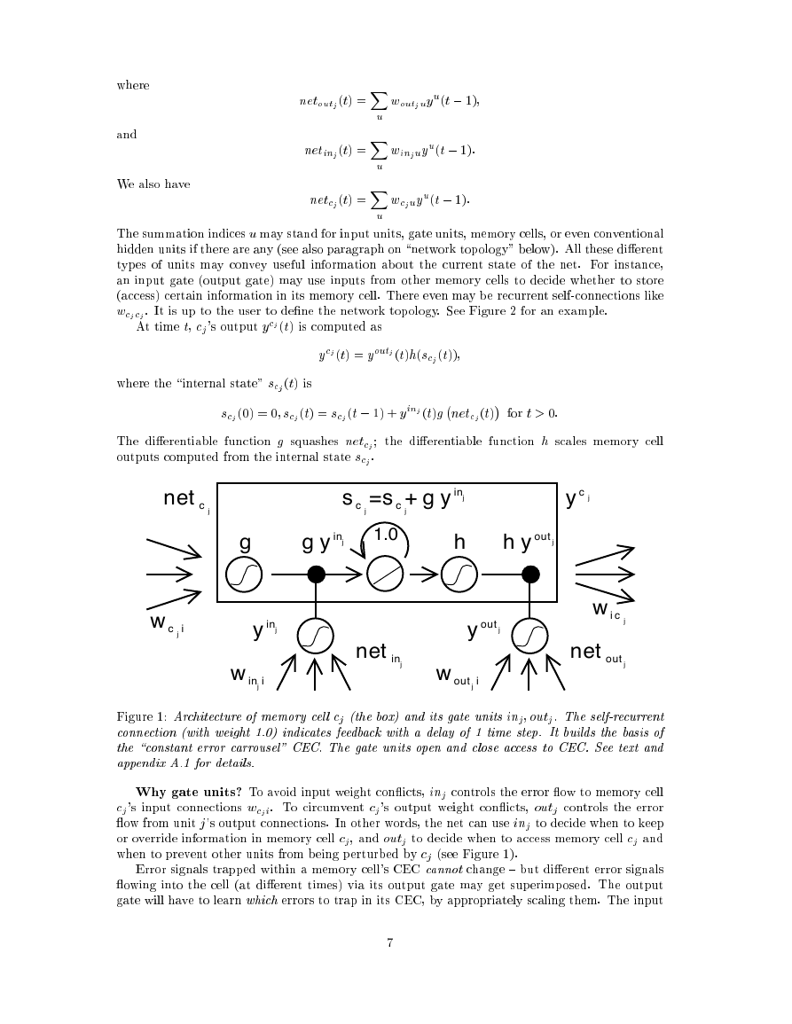
The resulting, more complex unit is called a memory cel l (see Figure �). The j -th memory cell
is denoted c
. Each memory cell is built around a central linear unit with a xed self-connection
j
(the CEC). In addition to net
, c
gets input from a multiplicative unit out
(the \output gate"),
c
j
j
j
and from another multiplicative unit in
(the \input gate"). in
's activation at time t is denoted
j
j
in
out
j
j
by y
(t), out
's by y
(t). We have
j
out
j
in
j
y
(t) = f
(net
(t)); y
(t) = f
(net
(t));
out
out
in
in
j
j
j
j
�
�
where
and
We also have
net
(t) =
w
y
(t �);
out
out
u
j
j
X
u
u
X
net
(t) =
w
y
(t �):
in
in
u
j
j
u
u
X
net
(t) =
w
y
(t �):
c
j
c
u
j
u
u
The summation indices u may stand for input units, gate units, memory cells, or even conventional
hidden units if there are any (see also paragraph on \network topology" below). All these dierent
types of units may convey useful information about the current state of the net. For instance,
an input gate (output gate) may use inputs from other memory cells to decide whether to store
(access) certain information in its memory cell. There even may be recurrent self-connections like
w
. It is up to the user to dene the network topology. See Figure � for an example.
c
c
j
j
At time t, c
's output y
(t) is computed as
j
c
j
c
out
j
j
y
(t) = y
(t)h(s
(t));
c
j
where the \internal state" s
(t) is
c
j
s
(�) = �; s
(t) = s
(t �) + y
(t)g
net
(t)
for t > �:
c
c
c
j
j
j
c
j
in
j
The dierentiable function g squashes net
; the dierentiable function h scales memory cell
c
j
outputs computed from the internal state s
.
c
j
net c j
s c j
g
g y inj
g+
=
s c j
1.0
y inj
h
y c j
h y out j
w ic j
y inj
w i
inj
net
inj
y out j
w i
out j
wi c j
net
out j
Figure �: Architecture of memory cel l c
(the box) and its gate units in
; out
. The self-recurrent
j
j
j
connection (with weight �.�) indicates feedback with a delay of � time step. It builds the basis of
the \constant error carrousel" CEC. The gate units open and close access to CEC. See text and
appendix A.� for details.
Why gate units? To avoid input weight conicts, in
controls the error ow to memory cell
j
c
's input connections w
. To circumvent c
's output weight conicts, out
controls the error
j
c
i
j
j
j
ow from unit j 's output connections. In other words, the net can use in
to decide when to keep
j
or override information in memory cell c
, and out
to decide when to access memory cell c
and
j
j
j
when to prevent other units from being perturbed by c
(see Figure �).
j
Error signals trapped within a memory cell's CEC cannot change { but dierent error signals
owing into the cell (at dierent times) via its output gate may get superimposed. The output
gate will have to learn which errors to trap in its CEC, by appropriately scaling them. The input
�
�
gate will have to learn when to release errors, again by appropriately scaling them. Essentially,
the multiplicative gate units open and close access to constant error ow through CEC.
Distributed output representations typically do require output gates. Not always are both
gate types necessary, though | one may be sucient. For instance, in Experiments �a and �b in
Section �, it will be possible to use input gates only. In fact, output gates are not required in case
of local output encoding | preventing memory cells from perturbing already learned outputs can
be done by simply setting the corresponding weights to zero. Even in this case, however, output
gates can be benecial: they prevent the net's attempts at storing long time lag memories (which
are usually hard to learn) from perturbing activations representing easily learnable short time lag
memories. (This will prove quite useful in Experiment �, for instance.)
Network topology. We use networks with one input layer, one hidden layer, and one output
layer. The (fully) self-connected hidden layer contains memory cells and corresponding gate units
(for convenience, we refer to both memory cells and gate units as being located in the hidden
layer). The hidden layer may also contain \conventional" hidden units providing inputs to gate
units and memory cells. All units (except for gate units) in all layers have directed connections
(serve as inputs) to all units in the layer above (or to all higher layers { Experiments �a and �b).
Memory cell blocks. S memory cells sharing the same input gate and the same output gate
form a structure called a \memory cell block of size S ". Memory cell blocks facilitate information
storage | as with conventional neural nets, it is not so easy to code a distributed input within a
single cell. Since each memory cell block has as many gate units as a single memory cell (namely
two), the block architecture can be even slightly more ecient (see paragraph \computational
complexity"). A memory cell block of size � is just a simple memory cell. In the experiments
(Section �), we will use memory cell blocks of various sizes.
Learning. We use a variant of RTRL (e.g., Robinson and Fallside � ��) which properly takes
into account the altered, multiplicative dynamics caused by input and output gates. However, to
ensure non-decaying error backprop through internal states of memory cells, as with truncated
BPTT (e.g., Williams and Peng � �), errors arriving at \memory cell net inputs" (for cell c
, this
j
includes net
, net
, net
) do not get propagated back further in time (although they do serve
c
in
out
j
j
j
to change the incoming weights). Only within
memory cells, errors are propagated back through
�
previous internal states s
. To visualize this: once an error signal arrives at a memory cell output,
c
j
�
it gets scaled by output gate activation and h
. Then it is within the memory cell's CEC, where it
can ow back indenitely without ever being scaled. Only when it leaves the memory cell through
the input gate and g , it is scaled once more by input gate activation and g
. It then serves to
�
change the incoming weights before it is truncated (see appendix for explicit formulae).
Computational complexity. As with Mozer's focused recurrent backprop algorithm (Mozer
� � ), only the derivatives
need to be stored and updated. Hence the LSTM algorithm is
@w
il
@ s
c
j
very ecient, with an excellent update complexity of O(W ), where W the number of weights (see
details in appendix A.�). Hence, LSTM and BPTT for fully recurrent nets have the same update
complexity per time step (while RTRL's is much worse). Unlike full BPTT, however, LSTM is
local in space and time
: there is no need to store activation values observed during sequence
�
processing in a stack with potentially unlimited size.
Abuse problem and solutions.
In the beginning of the learning phase, error reduction
may be possible without storing information over time. The network will thus tend to abuse
memory cells, e.g., as bias cells (i.e., it might make their activations constant and use the outgoing
connections as adaptive thresholds for other units). The potential diculty is:
it may take a
long time to release abused memory cells and make them available for further learning. A similar
\abuse problem" appears if two memory cells store the same (redundant) information. There are
at least two solutions to the abuse problem: (�) Sequential network construction (e.g., Fahlman
� �): a memory cell and the corresponding gate units are added to the network whenever the
For intra-cellular backprop in a quite dierent context see also Doya and Yoshizawa (� � ).
�
�
Following Schmidhuber (� � ), we say that a recurrent net algorithm is local in space if the update complexity
per time step and weight does not depend on network size. We say that a method is local in time if its storage
requirements do not depend on input sequence length. For instance, RTRL is local in time but not in space. BPTT
is local in space but not in time.
�
�



 2023年江西萍乡中考道德与法治真题及答案.doc
 2012年重庆南川中考生物真题及答案.doc
 2013年江西师范大学地理学综合及文艺理论基础考研真题.doc
 2020年四川甘孜小升初语文真题及答案I卷.doc
 2020年注册岩土工程师专业基础考试真题及答案.doc
 2023-2024学年福建省厦门市九年级上学期数学月考试题及答案.doc
 2021-2022学年辽宁省沈阳市大东区九年级上学期语文期末试题及答案.doc
 2022-2023学年北京东城区初三第一学期物理期末试卷及答案.doc
 2018上半年江西教师资格初中地理学科知识与教学能力真题及答案.doc
 2012年河北国家公务员申论考试真题及答案-省级.doc
 2020-2021学年江苏省扬州市江都区邵樊片九年级上学期数学第一次质量检测试题及答案.doc
 2022下半年黑龙江教师资格证中学综合素质真题及答案.doc