Mapping the World’s Photos
David Crandall, Lars Backstrom, Daniel Huttenlocher and Jon Kleinberg
Department of Computer Science
Cornell University
{crandall,lars,dph,kleinber}@cs.cornell.edu
Ithaca, NY
ABSTRACT
We investigate how to organize a large collection of geotagged pho-
tos, working with a dataset of about 35 million images collected
from Flickr. Our approach combines content analysis based on text
tags and image data with structural analysis based on geospatial
data. We use the spatial distribution of where people take photos
to define a relational structure between the photos that are taken at
popular places. We then study the interplay between this structure
and the content, using classification methods for predicting such
locations from visual, textual and temporal features of the photos.
We find that visual and temporal features improve the ability to
estimate the location of a photo, compared to using just textual fea-
tures. We illustrate using these techniques to organize a large photo
collection, while also revealing various interesting properties about
popular cities and landmarks at a global scale.
Categories and Subject Descriptors
H.2.8 [Database Management]: Database Applications—Data Min-
ing, Image Databases, Spatial Databases and GIS; I.4.8 [Image
Processing and Computer Vision]: Scene Analysis
General Terms
Measurement, Theory
Keywords
Photo collections, geolocation
1.
INTRODUCTION
Photo-sharing sites on the Internet contain billions of publicly-
accessible images taken virtually everywhere on earth (and even
some from outer space). Increasingly these images are annotated
with various forms of information including geolocation, time, pho-
tographer, and a wide variety of textual tags.
In this paper we
address the challenge of organizing a global collection of images
Supported in part by NSF grants CCF-0325453, CNS-0403340,
BCS-0537606, and IIS-0705774, and by funding from Google, Ya-
hoo!, and the John D. and Catherine T. MacArthur Foundation.
This research was conducted using the resources of the Cornell
University Center for Advanced Computing, which receives fund-
ing from Cornell University, New York State, NSF, and other public
agencies, foundations, and corporations.
Copyright is held by the International World Wide Web Conference Com-
mittee (IW3C2). Distribution of these papers is limited to classroom use,
and personal use by others.
WWW 2009, April 20–24, 2009, Madrid, Spain.
ACM 978-1-60558-487-4/09/04.
using all of these sources of information, together with the vi-
sual attributes of the images themselves. Perhaps the only other
comparable-scale corpus is the set of pages on the Web itself, and it
is in fact useful to think about analogies between organizing photo
collections and organizing Web pages. Successful techniques for
Web-page analysis exploit a tight interplay between content and
structure, with the latter explicitly encoded in hypertext features
such as hyperlinks, and providing an axis separate from content
along which to analyze how pages are organized and related [17].
In analyzing large photo collections, existing work has focused
primarily either on structure, such as analyses of the social network
ties between photographers (e.g., [7, 12, 14, 15, 24]), or on content,
such as studies of image tagging (e.g., [6, 18, 20]). In contrast our
goal is to investigate the interplay between structure and content —
using text tags and image features for content analysis and geospa-
tial information for structural analysis. It is further possible to use
attributes of the social network of photographers as another source
of structure, but that is beyond the scope of this work (although in
the conclusion we mention an interesting result along this vein).
The present work: Visual and geospatial information. The cen-
tral thesis of our work is that geospatial information provides an
important source of structure that can be directly integrated with
visual and textual-tag content for organizing global-scale photo col-
lections. Photos are inherently spatial — they are taken at specific
places — and so it is natural that geospatial information should
provide useful organizing principles for photo collections, includ-
ing map-based interfaces to photo collections such as Flickr [4].
Our claim goes beyond such uses of spatial information, however,
in postulating that geospatial data reveals important structural ties
between photographs, based on social processes influencing where
people take pictures. Moreover, combining this geospatial struc-
ture with content from image attributes and textual tags both re-
veals interesting properties of global photo collections and serves
as a powerful way of organizing such collections.
Our work builds on recent results in two different research com-
munities, both of which investigate the coupling of image and place
data. In the computer vision research community there has been
work on constructing rich representations from images taken by
many people at a single location [22, 23], as well as identifying
where a photo was taken based only on its image content [9]. In
the Web and digital libraries research community there has been
recent work on searching a collection of landmark images, using
a combination of features including geolocation, text tags and im-
age content [11]. While these previous investigations provide im-
portant motivation and some useful techniques for our work, they
do not provide methods for automatically organizing a corpus of
photos at global scale, such as the collection of approximately 35
million geotagged photos from Flickr that we consider here. As we
WWW 2009 MADRID!Track: Social Networks and Web 2.0 / Session: Photos and Web 2.0761�
see below, working at the level of all locations on earth requires
robust techniques for finding peaks in highly-multimodal distribu-
tions at different levels of spatial resolution, and computer vision
techniques that can capture rich image invariants while still scaling
to very large image corpora.
As researchers discovered a decade ago with large-scale collec-
tions of Web pages [13], studying the connective structure of a cor-
pus at a global level exposes a fascinating picture of what the world
is paying attention to. In the case of global photo collections, it
means that we can discover, through collective behavior, what peo-
ple consider to be the most significant landmarks both in the world
and within specific cities (see Table 2); which cities are most pho-
tographed (Table 1) which cities have the highest and lowest pro-
portions of attention-drawing landmarks (Table 4); which views of
these landmarks are the most characteristic (Figures 2 and 3); and
how people move through cities and regions as they visit different
locations within them (Figure 1). These resulting views of the data
add to an emerging theme in which planetary-scale datasets provide
insight into different kinds of human activity — in this case those
based on images; on locales, landmarks, and focal points scattered
throughout the world; and on the ways in which people are drawn
to them.
Location and content. One of the central goals of this work is to
study the relation between location and content in large photo col-
lections. In particular we consider the task of estimating where a
photo was taken based on its content, using both image attributes
and text tags. The authors of [9] investigate a similar question,
of determining GPS location using solely image content. In con-
trast to their work, our goal is to use location estimation as an ex-
perimental paradigm for investigating questions about the relative
value of image features and text tags in estimating location. More-
over, our definition of location is hierarchical and depends on where
people take photos, rather than just GPS coordinates.
We consider two spatial resolutions in defining locations:
the
metropolitan-area scale in which we resolve locations down to
roughly 100 kilometers, and the individual-landmark scale in which
we resolve locations down to roughly 100 meters. For ease of dis-
cussion we use the term landmark for the finer level even though
not all such locations would necessarily constitute “landmarks” in
the traditional sense of the term. At both scales, we determine im-
portant locations by using a mean shift procedure (see Section 3)
to identify locations with high densities of photos; these serve as
places whose locations we subsequently try to estimate by analyz-
ing the content of the photos at that place. Mean shift is particularly
applicable to the problem of finding highly photographed places,
because unlike most clustering techniques that require choosing
some number of clusters or making underlying distributional as-
sumptions, mean shift is a non-parametric technique that requires
only a scale of observation. We find that it is remarkably effective
on this type of data and at multiple scales.
In more detail, we take n geotagged photos from each of k au-
tomatically identified popular locations. Each photo has a number
of features including textual tags and image attributes (described
in Section 4.1) as well as one of the k geographic locations. We
separate the images into training and test sets (disjoint not only in
photos but also in photographers), suppress the geographic infor-
mation in the test set, and evaluate the performance of machine-
learning classification techniques on estimating the (hidden) loca-
tion for each photo in the test set.
For assessing the combination of visual information with textual
tags, one must take into account that text-tags are the single most
useful source of features for estimating hidden location values — a
reflection of the fact that current techniques are considerably more
effective at exploiting textual data than image data, and that pho-
tographers are generally able to provide more effective short textual
descriptions than can currently be extracted from raw image data
(e.g., [6, 20]).
Nonetheless, we find that at the landmark scale (100m) image
information is also very effective in estimating location. In a num-
ber of locales, its performance is only a little below that of textual
information (and always far above chance prediction), despite the
enormous variability in photo content in the photos taken at any
fixed location. Visual information also works well in combination
with other features. In particular, when visual information is com-
bined with temporal information — i.e., adding in visual features
from photos taken by the same photographers within a few-minute
window — it produces location estimates that are generally com-
parable to and sometimes above the performance of textual infor-
mation. Further, the combination of textual and visual information
yields significant improvements over text alone, and adding tempo-
ral information as well yields results that outperform any subset of
these features.
At the metropolitan scale (100km) text tags are again highly ef-
fective for estimating location, but the image features are no longer
useful; the image features alone perform at the level of chance,
and adding the image features to the text features does not improve
performance above the text features alone. This negative result pro-
vides further insight into the settings in which image characteristics
are most effective for this type of task — specifically, in dealing
with a corpus at a level of spatial resolution where there will be
many different images of the same thing. It thus suggests a natural
scale — at fairly short range — where the computational cost of us-
ing image-based techniques will produce the most significant pay-
off. It also suggests that the approach taken in [9], of using image
features alone to estimate global location, is not the most powerful
use of image content in organizing large photo collections.
Representative Images. Our second task considers the question
of what is being photographed at a given location, by selecting
representative images from a specific location. While visual in-
formation played a significant but supporting role in the first task,
it becomes the dominant factor here. Selecting canonical or rep-
resentative images is a problem that has a long history both in
perceptual psychology and computer vision. The majority of the
computational techniques are based on three-dimensional analysis
of the surfaces in a scene (e.g., [5]). Recently, with the advent of
Web photo collections, attention has been paid to generating canon-
ical views of a site based on popular places to take photos of that
site [22, 23]. This work again makes considerable use of three-
dimensional structure of the scene to infer where photos are taken
from. Our approach for this task is based heavily on this work,
with the important difference that we do not make use of the three-
dimensional scene constraints of that work. This results in a more
lightweight, faster overall process that is capable of scaling to the
global scope of our data, and yet which still produces considerably
better results than randomly selecting photos from a landmark lo-
cation, or even selecting photos based purely on textual tags.
Ultimately, the effectiveness of image-based features for this task
— and the ability of the methods to scale to large data sizes —
closes an important loop that is consistent with our overall goal and
in contrast to earlier smaller-scale studies: to show the potential
of applications that can provide overviews of global photo collec-
tions using absolutely no domain knowledge — no hand-selection
of cities or subsets of the corpus — but instead simply employing
a combination of raw usage, text, and image data available. (Fig-
WWW 2009 MADRID!Track: Social Networks and Web 2.0 / Session: Photos and Web 2.0762�
ures 2 and 3 are basic examples, in which the maps, the choice of
locations, the images, and the labels are all automatically inferred
from the Flickr corpus.)
2. DATASET
Our dataset was collected by downloading images and photo
metadata from Flickr.com using the site’s public API. Our goal was
to retrieve as large and unbiased a sample of geotagged photos as
possible. To do this, we first sample a photo id uniformly at random
from the space of Flickr photo id numbers, look up the correspond-
ing photographer, and download all the geotagged photos (if any)
of that initial user. For each photo we download metadata (tex-
tual tags, date and time taken, geolocation) and the image itself.
We then crawl the graph of contacts starting from this user, down-
loading all the geotagged photos. We repeat the entire process for
another randomly selected photo id number, keeping track of users
who have already been processed so that their photos and contact
lists are not re-crawled.
This crawl was performed during a six-month period in the sum-
mer and fall of 2008. In total we retrieved 60,742,971 photos taken
by 490,048 Flickr users. For the work in this paper we used a sub-
set of these photos for which the geolocation tags were accurate to
within about a city block (as reported by the Flickr metadata), con-
sisting of 33,393,835 photos by 307,448 users. The total size of the
database is nearly two terabytes.
3. FINDING AND CHARACTERIZING
LOCATIONS USING MEAN SHIFT
Given a large collection of geotagged photos we want to auto-
matically find popular places at which people take photos. In mea-
suring how popular a place is we consider the number of distinct
photographers who have taken a photo there, rather than the total
number of photos taken, in order to avoid pathologies associated
with the wide variability in photo-taking behavior across different
individuals.
Finding highly-photographed places can be viewed as a prob-
lem of clustering points in a two-dimensional feature space. For
instance [11] uses k-means clustering to find popular locations in
photo collections. k-means is a well-known example of a broad
class of fixed-cluster approaches that specify a number of clus-
ters in advance. Fixed-cluster approaches are particularly prob-
lematic for spatial data of the type we have, where extreme non-
uniformity occurs at many spatial scales. As an example, in our
dataset many of the largest clusters are in a few big cities such
as London, biasing fixed-cluster approaches away from the entire
globe and towards such areas. In their work, the authors of [11]
only apply fixed-cluster methods to a manually selected metropoli-
tan area (San Francisco); it would arguably be difficult to apply
this to discovering locations at high resolution over any larger scale
area.
Instead of fixed-cluster methods, we take advantage of the fact
that in spatial data there is a natural parameter based on scale of
observation. For instance, viewing a plot of photo locations at the
scale of a continent one will see clusters corresponding to cities
and metropolitan areas, whereas viewing the same data at the scale
of a single city one will see clusters corresponding to landmarks
and other points of interest. Thus we use mean shift clustering,
because this method requires only an estimate of the scale of the
data. While mean shift is often used for certain problems such as
image segmentation, it appears not to be as widely used in other
research areas.
Mean shift is a non-parametric technique for estimating the modes
of an underlying probability distribution from a set of samples,
given just an estimate of the scale of the data. In our setting, con-
ceptually there is an underlying unobservable probability distribu-
tion of where people take photographs, with modes corresponding
to interesting or important places to photograph. We are only able
to observe the locations at which people take photos, from which
mean shift allows us to estimate the modes of the underlying dis-
tribution. The mean shift approach is well-suited to highly multi-
modal probability density functions with very different mode sizes
and no known functional form, such as we have here.
Mean shift operates by directly estimating the gradient of the
probability density from the samples, in contrast with estimating
the density itself as is done with kernel density methods such as
Parzen windows. From zeroes of the gradient, local maxima of
the distribution can readily be determined. In fact the mean shift
calculation is an iterative procedure that uses the gradient estimate
as an update, so when the gradient vector is (near) zero magnitude
the procedure directly yields an estimate of the location of a local
maximum of the underlying distribution.
From a given location x the mean shift vector is defined as
mh,G(x) =
Pn
i=1 xig||(x − xi)/h||2
i=1 g||(x − xi)/h||2 − x
Pn
where the xi are observed data values, g are weights for each data
point corresponding to some chosen kernel function G (we use a
uniform function), and h is a bandwidth parameter. The mean shift
vector is simply the difference between the weighted mean, using
the kernel G, and x the center of the kernel.
The mean shift procedure computes a sequence starting from
some initial location x(1) where
x(i+1) = x(i) + mh,G(x(i))
which converges to a location that corresponds to a local maximum
of the underlying distribution as the mean shift vector approaches
zero. The convergence properties of mean shift are beyond the
scope of this paper, but the conditions are quite broad (see [2]).
Seeding this mean shift procedure from many initial points, the
trajectory from each starting point will converge to a mode of the
distribution (with a given mode often being the end-result of multi-
ple trajectories). In practice, the mean shift procedure can be made
very fast, particularly for low-dimensional data such as we have
here, through the use of bucketing techniques.
In our case we use the lat-long values in degrees for each photo,
treating them as points in the plane because the errors in doing
so are not substantial at the distances we consider. We bucket
the lat-long values at the corresponding spatial scale, 1 degree for
metropolitan-scale (100 km) and .001 degree for landmark-scale
(100 m). At a given scale, for each photographer we sample a sin-
gle photo from each bucket. We then perform the mean shift pro-
cedure at each scale separately, seeding by sampling a photo from
each bucket, using a uniform disc as the kernel.
We characterize the magnitude of each peak by simply counting
the number of points in the support area of the kernel centered at
the peak. This is effectively the number of distinct photographers
who took photos at that location (however may differ slightly as the
peaks do not align with the buckets used to sample a single photo
from each photographer).
Location clustering results. Table 1 presents the 15 most pho-
tographed metropolitan-scale peaks on Earth found via this mean
shift procedure, ranked according to number of distinct photogra-
phers. The table also shows selected lower-ranked peaks by rank.
The textual description of each cluster was generated automatically
WWW 2009 MADRID!Track: Social Networks and Web 2.0 / Session: Photos and Web 2.0763�
Earth
Top landmark
eiffel
2nd landmark
trafalgarsquare
3rd landmark
tatemodern
4th landmark
bigben
5th landmark
notredame
6th landmark
londoneye
7th landmark
empirestatebuilding
empirestatebuilding
trafalgarsquare
coittower
eiffel
disneyland
cloudgate
1. newyorkcity
2. london
3. sanfrancisco
4. paris
5. losangeles
6. chicago
7. washingtondc washingtonmonument wwii
8. seattle
9. rome
timessquare
tatemodern
pier39
notredame
hollywood
chicagoriver
10. amsterdam
11. boston
12. barcelona
13. sandiego
14. berlin
15. lasvegas
16. firenze
17. toronto
18. milano
19. vancouver
20. madrid
21. venezia
22. philadelphia
23. austin
24. dublin
25. portland
spaceneedle
colosseum
dam
fenwaypark
sagradafamilia
balboapark
brandenburgertor
paris
pontevecchio
cntower
duomo
granvilleisland
plazamayor
sanmarco
libertybell
capital
oconnellstreet
pioneersquare
rockefeller
bigben
unionsquare
louvre
gettymuseum
hancock
lincolnmemorial
seattlepubliclibrary gasworkspark
fontanaditrevi
pantheon
amsterdam
nieuwmarkt
publicgarden
faneuilhall
cathedral
boqueria
seals
ussmidway
potsdamerplatz
berlinerdom
venetian
bellagio
firenze
piazzadelcampo
rom
colonne
market
vaticano
westerkerk
trinitychurch
parcguell
sandiegozoo
reichstag
newyorknewyork
duomo
nathanphillipssquare dundassquare
castellosforzesco
vancouverartgallery vancouveraquarium downtown
puertadelsol
rialto
artmuseum
emos
bridge
powells
cibeles
canal
cityhall
sxsw
dublin
saturdaymarket
cathedral
italy
logancircle
sxsw
dublincastle
chinesegarden
centrale
grandcentralstation applestore
londoneye
ferrybuilding
sacrecoeur
frankgehry
searstower
capitol
columbuscircle
buckingham
lombardstreet
centrepompidou
griffithobservatory
wrigleyfield
libertyisland
towerbridge
sanfrancisco
trocadero
californiaadventure
buckinghamfountain
whitehouse
fountain
vittoriano
europe
piccadillycircus
prison
arcdetriomphe
santamonicapier
artinstitute
jeffersonmemorial museum
kerrypark
basilica
museumplein
usa
casamilà
sandiegopadres
tvtower
casino
santacroce
eatoncentre
cordusio
gastown
callao
venice
citizensbankpark
sxswi
trinity
japanesegarden
downtown
spanishsteps
europe
newenglandaquarium harvardyard
spain
starofindia
gedächtniskirche
flamingo
bridge
unionstation
duomo
englishbay
metropolis
venice
rittenhouse
tower
christchurch
fountain
casabatlló
comiccon
checkpointcharlie
luxor
river
hockeyhalloffame
sanbabila
clock
parquedelretiro
italia
centercity
southcongress
storehouse
pdx
Table 2: The seven most photographed landmarks on Earth, and the top seven landmarks in each of the top 25 metropolitan-scale
areas, found using mean-shift clustering.
Rank Users Photos Most distinctive tags
586203 paris france
775061 losangeles california
515884 chicago illinois
571698 washingtondc dc washington
535671 seattle washington
243726 rome roma italy italia
280549 amsterdam holland netherlands
402658 boston massachusetts
258926 barcelona spain
304720 sandiego california
236818 berlin germany
206670 lasvegas vegas nevada
112204 firenze florence italy italia tuscany toscana
164454 madrid spain españa
156693 montreal canada quebec
131367 hongkong china
122972 pittsburgh pennsylvania
1 35860 1204137 newyorkcity nyc newyork
2 29152 1122476 london england
3 25694 1115870 sanfrancisco california
4 18940
5 17729
6 12025
7 11834
8 11346
9839
9
9607
10
9318
11
9229
12
13
9132
8369
14
7652
15
7438
16
6586
20
47
3620
2731
61
2312
73
1591
121
1308
151
202
951
579
301
383
374
291
441
139
640
85
800
933
58
49
1000
9580 nassau atlantis bahamas cruise
4254 juneau glacier alaska
2411 beirut lebanon
3525 galapagos wildlife galapagosislands ecuador
20319 yellowstonenationalpark yellowstone wyoming
61971 mexicocity df mexico
27754 ithaca newyork ny
19551 iowacity iowa
709 laketiticaca southamerica titicaca uros peru puno
608 bialystok białystok poland polska
Table 1: Clustering results at the metropolitan-scale, showing
the most photographed places on Earth ranked by number of
distinct photographers.
Most salient
58.2 agra tajmahal
49.4 córdoba cordoba
46.4 dubrovnik croatia
45.7 salamanca españa
44.2 blackrockcity burningman
42.0 ljubljana slovenia
38.5 corpuschristi texas
34.6 montsaintmichel saintmalo
33.5 grandcanyon grand
32.8 deathvalley death
31.8 firenze florence
31.8 kraków krakow
31.7 habana havana
31.1 venezia venice
29.9 jerusalem israel
29.7 praha prague
28.7 keywest key
28.2 chattanooga tennessee
28.0 rome roma
27.9 trogir split
Least salient
6.1 desmoines iowa
6.1 minneapolis minnesota
6.0 fremantle perth
6.0 bern suisse
5.9 rochester ny
5.9 brisbane queensland
5.9 frankfurt germany
5.8 brest finistère
5.8 amsterdam holland
5.7 newcastle durham
5.7 taichung taiwan
5.5 santiago chile
5.4 sanfrancisco california
5.0 maastricht aachen
4.9 adachi arakawa
4.7 miami florida
4.6 connecticut ct
4.1 hannover deutschland
3.7 graubünden schweiz
3.4 taipei taiwan
Table 4: Cities ranked according to saliency of landmarks.
WWW 2009 MADRID!Track: Social Networks and Web 2.0 / Session: Photos and Web 2.0764�
City
Baseline
Textual tags Visual tags Combined
Textual tags Visual tags Combined
Single photos
Temporal
1. newyorkcity
2. london
3. sanfrancisco
4. paris
5. losangeles
6. chicago
7. washingtondc
8. seattle
9. rome
10. amsterdam
Cities 1-10
Cities 41-50
Cities 91-100
Cities 1-100
Cities 1-10 (25-way)
Cities 1-10 (50-way)
10.00
10.00
10.00
10.00
10.00
10.00
10.00
10.00
10.00
10.00
10.00
10.00
10.00
10.00
4.00
2.00
50.90
55.96
53.49
50.30
58.76
55.86
48.01
56.36
44.73
34.96
51.67
46.91
38.87
44.57
44.64
38.16
44.52
42.96
37.76
45.34
33.33
42.40
42.17
38.92
47.56
24.00
41.63
34.15
26.58
30.59
23.56
14.40
66.41
67.71
63.96
64.84
63.10
66.81
61.55
65.11
62.97
39.02
63.86
55.25
44.27
51.71
51.11
41.85
52.98
57.12
56.37
51.48
60.54
58.54
49.43
58.72
45.14
36.13
53.21
48.12
39.84
45.70
45.90
39.53
54.69
52.27
52.04
56.74
44.80
51.73
53.33
50.66
58.63
28.87
52.55
42.88
30.29
37.57
30.11
20.56
70.28
70.38
70.64
69.04
65.73
70.36
65.28
69.14
66.74
42.80
67.81
58.08
46.18
54.06
53.16
43.96
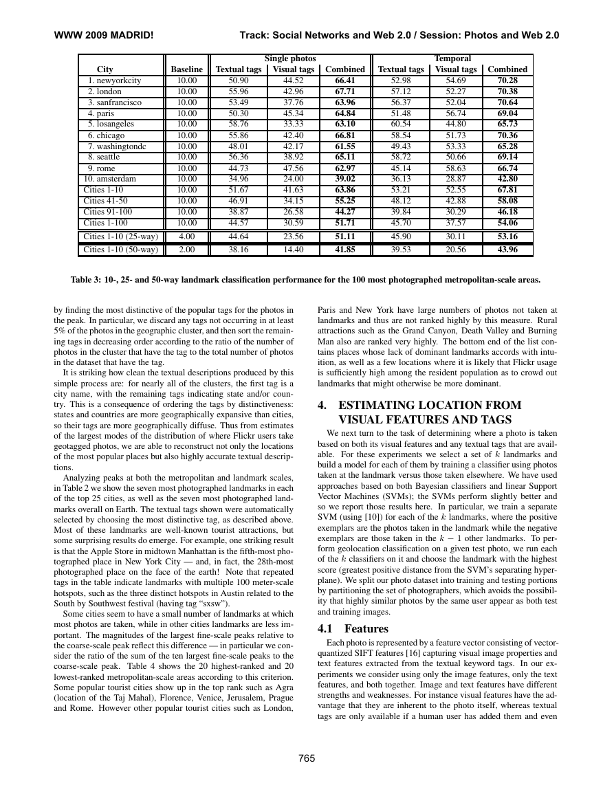
Table 3: 10-, 25- and 50-way landmark classification performance for the 100 most photographed metropolitan-scale areas.
by finding the most distinctive of the popular tags for the photos in
the peak. In particular, we discard any tags not occurring in at least
5% of the photos in the geographic cluster, and then sort the remain-
ing tags in decreasing order according to the ratio of the number of
photos in the cluster that have the tag to the total number of photos
in the dataset that have the tag.
It is striking how clean the textual descriptions produced by this
simple process are: for nearly all of the clusters, the first tag is a
city name, with the remaining tags indicating state and/or coun-
try. This is a consequence of ordering the tags by distinctiveness:
states and countries are more geographically expansive than cities,
so their tags are more geographically diffuse. Thus from estimates
of the largest modes of the distribution of where Flickr users take
geotagged photos, we are able to reconstruct not only the locations
of the most popular places but also highly accurate textual descrip-
tions.
Analyzing peaks at both the metropolitan and landmark scales,
in Table 2 we show the seven most photographed landmarks in each
of the top 25 cities, as well as the seven most photographed land-
marks overall on Earth. The textual tags shown were automatically
selected by choosing the most distinctive tag, as described above.
Most of these landmarks are well-known tourist attractions, but
some surprising results do emerge. For example, one striking result
is that the Apple Store in midtown Manhattan is the fifth-most pho-
tographed place in New York City — and, in fact, the 28th-most
photographed place on the face of the earth! Note that repeated
tags in the table indicate landmarks with multiple 100 meter-scale
hotspots, such as the three distinct hotspots in Austin related to the
South by Southwest festival (having tag “sxsw”).
Some cities seem to have a small number of landmarks at which
most photos are taken, while in other cities landmarks are less im-
portant. The magnitudes of the largest fine-scale peaks relative to
the coarse-scale peak reflect this difference — in particular we con-
sider the ratio of the sum of the ten largest fine-scale peaks to the
coarse-scale peak. Table 4 shows the 20 highest-ranked and 20
lowest-ranked metropolitan-scale areas according to this criterion.
Some popular tourist cities show up in the top rank such as Agra
(location of the Taj Mahal), Florence, Venice, Jerusalem, Prague
and Rome. However other popular tourist cities such as London,
Paris and New York have large numbers of photos not taken at
landmarks and thus are not ranked highly by this measure. Rural
attractions such as the Grand Canyon, Death Valley and Burning
Man also are ranked very highly. The bottom end of the list con-
tains places whose lack of dominant landmarks accords with intu-
ition, as well as a few locations where it is likely that Flickr usage
is sufficiently high among the resident population as to crowd out
landmarks that might otherwise be more dominant.
4. ESTIMATING LOCATION FROM
VISUAL FEATURES AND TAGS
We next turn to the task of determining where a photo is taken
based on both its visual features and any textual tags that are avail-
able. For these experiments we select a set of k landmarks and
build a model for each of them by training a classifier using photos
taken at the landmark versus those taken elsewhere. We have used
approaches based on both Bayesian classifiers and linear Support
Vector Machines (SVMs); the SVMs perform slightly better and
so we report those results here. In particular, we train a separate
SVM (using [10]) for each of the k landmarks, where the positive
exemplars are the photos taken in the landmark while the negative
exemplars are those taken in the k − 1 other landmarks. To per-
form geolocation classification on a given test photo, we run each
of the k classifiers on it and choose the landmark with the highest
score (greatest positive distance from the SVM’s separating hyper-
plane). We split our photo dataset into training and testing portions
by partitioning the set of photographers, which avoids the possibil-
ity that highly similar photos by the same user appear as both test
and training images.
4.1 Features
Each photo is represented by a feature vector consisting of vector-
quantized SIFT features [16] capturing visual image properties and
text features extracted from the textual keyword tags. In our ex-
periments we consider using only the image features, only the text
features, and both together. Image and text features have different
strengths and weaknesses. For instance visual features have the ad-
vantage that they are inherent to the photo itself, whereas textual
tags are only available if a human user has added them and even
WWW 2009 MADRID!Track: Social Networks and Web 2.0 / Session: Photos and Web 2.0765�
then can be irrelevant to geoclassification. On the other hand, au-
tomatically finding and interpreting visual features is much more
challenging than interpreting textual tags.
Visual features. Invariant interest point detection has become a
popular technique for handling the dramatic variations in object ap-
pearance from one image to another. The idea is to identify salient
keypoints that are likely to be stable across a range of image trans-
formations such as scaling, rotation, and perspective distortion –
corners, for example. For each interest point a descriptor is also
computed that characterizes the local image region in an invariant
way. We use keypoints detected by SIFT [16], which is among
the most popular feature point detectors in the recent computer vi-
sion literature. SIFT works by convolving an image with a bank of
Laplacian of Gaussian filters at several different scales, and iden-
tifying image points that are extrema in both the spatial and scale
dimensions of the filter bank response. A subsequent verification
step removes points along image edges and in noisy low-contrast
regions. Finally, an invariant descriptor is computed based on the
filter bank response and estimated local scale and orientation.
For a typical image, SIFT produces several hundred feature points.
The SIFT descriptor for each keypoint is a 128-dimensional vector
and has been found to be a highly distinctive representation of the
local image data [16]. While the visual similarity of a pair of im-
ages can be measured by comparing all pairs of SIFT descriptors
across the two images to find the most similar matching ones, this
does not scale well (for instance, [11] does not use SIFT features
for searching photo collections because of the computational cost).
A more scalable approach, taken in the object category recogni-
tion literature, is to use all the SIFT features in the training set to
create a “visual vocabulary” by vector quantization, generally us-
ing k-means. In our experiments we use k = 1000 and as in [3]
we sample a fixed number of keypoints per image, so that photos
with a large number of feature points are not represented dispro-
portionately during the clustering. The result is a set of 1,000 “vi-
sual keywords” with which we can label an image. Each image
is then represented by a 1000-dimensional vector indicating how
many times each SIFT “keyword” occurs in the image. That is, to
produce the feature vector for an image, we run the SIFT detector
and then find its visual words by locating the closest cluster in our
vocabulary for each of the detected interest points in the image.
We extracted the visual features from photos at Flickr’s medium-
scale image resolution, which is about 500 pixels on the larger
dimension. We found this image size to offer a good compro-
mise between performance and computational cost: using higher-
resolution images (1000 pixels on the larger dimension) did not
improve classification results significantly, while thumbnail images
(100 pixels on the larger dimension) were very fast but lowered
classification results by 10-20 percentage points. We also tried aug-
menting the local SIFT-based features with more global scene-level
visual features using the Gist operator [19], but found that this did
not improve our results significantly.
Textual features. We encode the textual features using a simple
unweighted vector space model. Any textual tag occurring in more
than 2 training exemplars is included as a dimension of the feature
vector (a multi-word tag corresponds to a single dimension). Tags
occurring 2 or fewer times are ignored, as they are seldom useful for
geolocation. If a given image includes a given tag, then the entry
in the corresponding feature vector is a 1 and otherwise it is a 0.
The dimensionality of the feature vectors depends on the number
of distinct tags that are found in the training set, but is typically
between 500 and 3,000 in our experiments.
Geolocation results. Table 3 presents classification results for the
ten most photographed landmark-scale locations in each of ten most
photographed metropolitan-scale regions. In each case the task is to
classify photos according to which of ten possible landmark-scale
locations they were taken in. To simplify interpretation of the re-
sults, the test sets were constructed so that each of the landmarks
had an equal number of photos; thus simply guessing uniformly at
random achieves a baseline classification rate of 10% correct. The
table shows that the correct classification rate using textual tags
varies from region to region, but is typically 4-6 times better than
the baseline. Using visual tags alone performs considerably worse
than using textual tags, but still outperforms the baseline by a fac-
tor of about 3 or 4. That visual tags underperform textual tags is to
be expected, considering that computationally extracting meaning
from visual features remains a challenging problem. The classifica-
tion rate differences between the baselines, visual classifier, textual
classifier, and combined classifier were all statistically significant
at p < 0.00001 according to Fisher’s Sign Test.
It is somewhat surprising that, despite the power of text features
alone over visual features alone, the two together outperform text
features alone by a significant margin. Some of this performance
gain is because some images do not have textual tags (as not all
photographers add them) whereas all images by definition have vi-
sual features. For example, of the New York City photos (the first
row of Table 3), 14% have no textual tags; and in fact if these pho-
tos are excluded from the test set, the performance of the textual
features on the remaining photos jumps from 50.90% to 62.51%.
However even on this set where all images have tags, visual fea-
tures still improve performance over tags alone, increasing accu-
racy from 62.51% to 71.34%. This illustrates that visual features
are useful even when people have added explicit textual tags to all
the photos.
We conducted this 10-way landmark classification task for each
of the top 100 cities, in an experiment that involved a total of over
two million test and training images. The results are shown in
the lower portion of Table 3. The conclusions of this experiment
echo those observed above for individual cities: textual tags per-
form nearly 5 times better than chance, visual tags perform 3 times
as well as chance, and the combination of features performs better
than either does individually. As shown in the table, the perfor-
mance on higher-ranked cities is generally better than on lower-
ranked cities which is in part due to the greater number of training
exemplars that are available in larger cities. (For example, the clas-
sification results for Amsterdam are poor because although it is the
tenth-most photographed city, relatively few photos are taken in
its top ten landmarks, as reflected by its low saliency score in Ta-
ble 4.) However this also raises the interesting possibility that there
are certain properties of the more highly photographed cities that
make them more easily classifiable visually.
Table 3 also shows results for the 25- and 50-way landmark clas-
sification task for the top 10 cities. The performance of the visual
classifier degrades roughly linearly as the number of landmarks in-
creases, or about 4-6 times better than chance. Surprisingly, the
textual and combined classifiers degrade quite slowly relative to
the baseline; at 50 landmarks, the classifier performs more than 20
times better than chance. We do not report results for all 100 cities
because most of the lower-ranked cities do not have a sufficient
number of Flickr photos at their less salient landmark locations.
An analogous experiment can be performed for the top landmark-
scale locations of Earth (which are listed on the first line of Table 2).
For ten landmarks, the classification performance is 69.39% using
text features, 46.28% using image features and 79.59% using the
two combined; for fifty landmarks, the respective correct classifica-
WWW 2009 MADRID!Track: Social Networks and Web 2.0 / Session: Photos and Web 2.0766�
tion rates are 52.67%, 25.43%, and 59.39% (the latter of which is
nearly 30 times better than the baseline). It is perhaps not surpris-
ing that text tags are even more valuable here, as tags such as the
name of a city or country are more informative when the landmarks
are geographically disparate. On the other hand the visual features
perform comparably on this problem as for the metropolitan-scale
problems, suggesting that landmarks across the globe are not visu-
ally more distinctive than those within a given city.
Finally we consider the ability to estimate the location of more
geographically disperse areas than specific landmarks. We use the
same training and classification paradigm, but for clusters of pho-
tos at the metropolitan-scale rather than the landmark-scale. Tex-
tual tag features remain quite distinctive at this scale and hence
perform well, giving a correct classification rate of 56.83% on the
10-way problem. Visual features, on the other hand, are not use-
ful, performing comparably to chance (12.72%) on their own and
not improving the text-only results when used in combination. This
result is intuitive: there is relatively little that visually separates a
typical scene in one city from a typical scene in another. These re-
sults support the use of image features for classification of spatially
local landmarks rather than identifying where on the globe photos
were taken.
5. ADDING TEMPORAL INFORMATION
Time provides another dimension along which photographs can
be connected together. That photos are taken at the same time is
not in itself a strong connection – dozens of unrelated photos are
taken within seconds of one another in our dataset. However, pho-
tos taken at nearby places at nearly the same time are very likely to
be related. In this section we show that temporal information can
be exploited both to recover interesting facts about human behavior,
and to geolocate photos more accurately.
Sequences of photos for which we know both the location and
time of capture can give fascinating insight into the way that people
move and interact. Geotagged and timestamped photos on Flickr
create something like the output of a rudimentary GPS tracking de-
vice: every time a photo is taken, we have an observation of where
a particular person is at a particular moment of time. By aggre-
gating this data together over many people, we can reconstruct the
typical pathways that people take as they move around a geospatial
region. For example, Figure 1 shows such diagrams for Manhat-
tan and the San Francisco Bay area. To produce these figures, we
plotted the geolocated coordinates of sequences of images taken by
the same user, sorted by time, for which consecutive photos were
no more than 30 minutes apart. We also discarded outliers caused
by inaccurate timestamps or geolocations. In the figure we have
superimposed the resulting diagrams on city maps for ease of visu-
alization.
The figures are striking in the amount of detail they reveal about
these cities. For example, one can clearly see the grid structure of
the Manhattan streets, caused by users traveling and taking photos
along them. The Brooklyn Bridge, in the lower center of the figure,
is clearly visible, as are the Manhattan and Williamsburg bridges
just to the north. One can even see the route of the ferries that take
tourists from Lower Manhattan to the Statue of Liberty.
Improving classification performance. Given the strong connec-
tion between space, time, and images, it is natural to revisit the
landmark classification problem of the last section, adding tempo-
ral information in addition to the textual and visual features. We
integrate temporal information directly into the classification pro-
cedure as follows. In classifying a photo, we also examine the pho-
tos taken by the same photographer within 15 minutes before and
after the picture was taken. For each of these photos, we compute
the classification distances for each of the k SVM classifiers, sum
the scores from the different images together to produce a single k-
vector, and then make the classification decision using that vector.
The motivation behind this simple technique is that photos taken
within a short period of time are often different shots of the same
landmark. Thus the textual and visual features of contemporaneous
photos are likely to be relevant in performing landmark classifica-
tion.
Table 3 compares the performance on the landmark classification
task with and without using this temporal information. For the clas-
sifiers that use only textual tags, the improvement is small (though
statistically significant, at p < 0.00001): many Flickr users appear
to label groups of consecutive photos with the same tags, and so
tags from contemporaneous frames do not provide much additional
information. For the visual tags, however, temporal information
improves the results dramatically. In the case of New York City,
for example, the improvement is over ten percentage points. This
is also an intuitive result, though striking in the actual magnitude
of the performance gain: photographers take multiple pictures of
the same landmark in order to capture different viewpoints, light-
ing conditions, subjects, etc., and thus neighboring frames provide
nonredundant visual evidence of where the photos were taken. In
fact, for several of the cities including New York, Paris, Washing-
ton, and Rome, the temporal-visual features actually outperform
the temporal-textual tag features. For all of the cities the best per-
formance is achieved by using the full combination of textual, vi-
sual, and temporal information.
6. REPRESENTATIVE IMAGES
Given our ability to automatically find and generate textual de-
scriptions of cities and landmarks, it is natural to ask whether it is
possible to extract visual descriptions as well. That is, given a set
of photos known to be taken near a landmark, we wish to automat-
ically select a canonical image of the landmark. This problem is
non-trivial because the subject of most photos taken near a land-
mark is actually not the landmark itself, so simple techniques like
random selection do very poorly.
To choose a canonical image we once again exploit the informa-
tion revealed by the collective behavior of Flickr users. People take
photos because they think a subject is visually interesting, pleasing,
or distinctive: it is as if photos of a landmark are votes for what the
visual representation of the landmark should be. Thus we find rep-
resentative images by looking for subsets of photos that are visually
very similar, and choosing an image from among the most salient
subset.
As in [22], we pose canonical image selection as a graph prob-
lem. We construct a graph in which each node represents a photo
and between each pair of nodes is an edge with a weight indicating
the degree of visual similarity between the two photos. Our goal
is then to find a tightly-connected cluster of photos that are highly
similar. To do this we use a spectral clustering technique [21] that
partitions the nodes of the graph using the second eigenvector of
the graph’s Laplacian matrix. Finally, we choose as the canonical
image for each cluster the one corresponding to the node with the
largest weighted degree.
The main difference between our approach and that of [22] is that
we are not interested in reconstructing or using detailed 3-d infor-
mation about a landmark, but rather in finding canonical images for
each landmark among vast amounts of data. Thus we use an image
similarity technique that is less precise than their method, in that it
does not enforce any 3d-geometric consistency, but is computation-
ally feasible for thousands of landmarks with thousands of photos
WWW 2009 MADRID!Track: Social Networks and Web 2.0 / Session: Photos and Web 2.0767�
Figure 1: Visualization of photographer movement in Manhattan and the San Francisco Bay area.
per landmark. Following [22] we extract SIFT interest points and
descriptors from each image. We then simply use the number of
“matching” interest points between a pair of images as a measure
of similarity, where matches are determined using the Euclidean
distance between SIFT descriptors.
Figures 2 and 3 present maps of representative images for the
top landmark in each of the top 20 North American and European
cities. All parts of the map were generated automatically using the
techniques presented in this paper: the metropolitan- and landmark-
sized clusters were found using the mean shift technique of Sec-
tion 3, the textual descriptions were formed by concatenating the
most distinctive textual tag of the landmark with that of the city,
and the representative images were chosen using the method pre-
sented in this section. Even the map itself was drawn automatically,
by simply plotting the raw latitudes and longitudes of all photos
geotagged within North America. The result is a strikingly accu-
rate map of the continent: land boundaries are easily recognizable
(presumably due to the large number of photos taken at beaches),
and one can easily see hotspots of photo activity corresponding to
cities and even major transportation arteries (such as the interstate
highways crossing the U.S. from east to west). Thus we see that
while individual users of Flickr are simply using the site to store
and share photos, their collective activity reveals a striking amount
of geographic and visual information about the world.
We have generated representative images for many of the top
cities and landmarks of the world; these results are available at
http://www.cs.cornell.edu/~crandall/photomap/.
7. RELATED WORK
Our work is motivated by and builds on recent results both in the
computer vision research community and in the Web and digital
libraries research community (as already mentioned in the previ-
ous sections). In particular we take much of our motivation from
the work of [9] and [11]; both of these papers have similar goals
of combining geospatial information with content for organizing
photo collections, with the former paper considering just image
content and the latter considering both images and text tags. While
pioneering papers, these works each have limitations that prevent
them from being scaled up even to the tens of millions of images
from around the globe that we consider here, much less the hun-
dreds of millions of geotagged images on photo sharing sites.
In [9] the authors propose the challenging problem of estimating
where a photo was taken based only on its image content. They cre-
ate a dataset of over 6 million geotagged photos by searching photo
sharing sites for tags such as names of cities and tourist sites. They
then characterize each photo using a number of image features such
as the gist operator [19], color and line features, and scene attributes
such as surface orientations. They then manually choose a set of
237 test images taken by photographers whose photos were not in-
cluded in the previous dataset. Using nearest-neighbor techniques
on vectors composed of the image features, they estimate a location
for each test image and measure the error compared to the (hidden)
true location. They find that this results in substantial improvement
compared to a random-guessing baseline, although the actual mag-
nitudes of the spatial errors are generally quite large for any practi-
cal application to photo organization. While [9] uses a set of over 6
million images, it is difficult to conclude how general their results
are because they are based only on 237 hand-selected photos, and
their methods do not scale to large evaluation sets. In contrast we
automatically find thousands of interesting locations, see how well
each can be localized using both image properties and text proper-
ties alone and together, and report statistically significant results.
In [11] the authors address the problem of searching a collection
of geolocated images, using a combination of spatial, text tag and
image content features. While like our work they consider the rela-
tive value of text tags versus image attributes for localization, their
methodology is based on qualitative user assessments of just 10 lo-
cations in a single geographic area (San Francisco) and using only
WWW 2009 MADRID!Track: Social Networks and Web 2.0 / Session: Photos and Web 2.0768�







 2023年江西萍乡中考道德与法治真题及答案.doc
 2012年重庆南川中考生物真题及答案.doc
 2013年江西师范大学地理学综合及文艺理论基础考研真题.doc
 2020年四川甘孜小升初语文真题及答案I卷.doc
 2020年注册岩土工程师专业基础考试真题及答案.doc
 2023-2024学年福建省厦门市九年级上学期数学月考试题及答案.doc
 2021-2022学年辽宁省沈阳市大东区九年级上学期语文期末试题及答案.doc
 2022-2023学年北京东城区初三第一学期物理期末试卷及答案.doc
 2018上半年江西教师资格初中地理学科知识与教学能力真题及答案.doc
 2012年河北国家公务员申论考试真题及答案-省级.doc
 2020-2021学年江苏省扬州市江都区邵樊片九年级上学期数学第一次质量检测试题及答案.doc
 2022下半年黑龙江教师资格证中学综合素质真题及答案.doc