This article has been accepted for inclusion in a future issue of this journal. Content is final as presented, with the exception of pagination.
IEEE TRANSACTIONS ON AUTOMATION SCIENCE AND ENGINEERING
1
Monocular Visual–Inertial State Estimation With
Online Initialization and Camera–IMU
Extrinsic Calibration
Zhenfei Yang, Student Member, IEEE, and Shaojie Shen, Member, IEEE
Abstract— There have been increasing demands for developing
microaerial vehicles with vision-based autonomy for search and
rescue missions in complex environments. In particular, the
monocular visual–inertial system (VINS), which consists of only
an inertial measurement unit (IMU) and a camera, forms a
great lightweight sensor suite due to its low weight and small
footprint. In this paper, we address two challenges for rapid
deployment of monocular VINS: 1) the initialization problem
and 2) the calibration problem. We propose a methodology that
is able to initialize velocity, gravity, visual scale, and camera–IMU
extrinsic calibration on the fly. Our approach operates in natural
environments and does not use any artificial markers. It also
does not require any prior knowledge about the mechanical
configuration of the system. It is a significant step toward plug-
and-play and highly customizable visual navigation for mobile
robots. We show through online experiments that our method
leads to accurate calibration of camera–IMU transformation,
with errors less than 0.02 m in translation and 1° in rotation.
We compare out method with a state-of-the-art marker-based
offline calibration method and show superior results. We also
demonstrate the performance of the proposed approach in large-
scale indoor and outdoor experiments.
Note to Practitioners—This paper presents a methodology for
online state estimation in natural environments using only a cam-
era and a low-cost micro-electro-mechanical systems (MEMS)
IMU. It focuses on addressing the problems of online estimator
initialization, sensor extrinsic calibration, and nonlinear opti-
mization with online refinement of calibration parameters. This
paper is particularly useful for applications that have superior
size, weight, and power constraints. It aims for rapid deployment
of robot platforms with robust state estimation capabilities with
Manuscript received January 3, 2016; accepted March 10, 2016. This paper
was recommended for publication by Associate Editor A. M. Hsieh and Editor
Y. Sun upon evaluation of the reviewer’s comments. This work was supported
in part by the Hong Kong University of Science and Technology under
Grant R9341. This paper is a revised and extended version of “Monocular
Visual-Inertial Fusion with Online Initialization and Camera-IMU Calibration”
presented at
the IEEE International Symposium on Safety, Security, and
Rescue Robotics, West Lafayette, IN, USA, October 2015.
The authors are with the Department of Electronic and Computer Engineer-
ing, Hong Kong University of Science and Technology, Hong Kong (e-mail:
zyangag@connect.ust.hk; eeshaojie@ust.hk).
This paper has supplementary downloadable multimedia material available
at http://ieeexplore.ieee.org provided by the authors. The Supplementary
Material contains the following. Three experiments are presented in the video
to demonstrate the performance of our self-calibrating monocular visual-
inertial state estimation method. The first experiment details the camera-
IMU extrinsic calibration process in a small indoor experiment. The second
experiment evaluates the performance of the overall system in a large-scale
indoor environment with highlights to the online calibration process. The
third experiment presents the state estimation results in a large-scale outdoor
environment using different camera configurations. This material is 52.6 MB
in size.
Color versions of one or more of the figures in this paper are available
online at http://ieeexplore.ieee.org.
Digital Object Identifier 10.1109/TASE.2016.2550621
almost no setup, calibration, or initialization overhead. The
proposed method can be used in platforms including handheld
devices, aerial robots, and other small-scale mobile platforms,
with applications in monitoring,
inspection, and search and
rescue.
Index Terms— Calibration, estimator initialization,
sensor
visual–inertial
fusion,
systems (VINSs).
state
estimation,
visual navigation,
I. INTRODUCTION
THERE have been increasing demands for developing
high maneuverability robots, such as microaerial vehi-
cles (MAVs) with vision-based autonomy for search and rescue
missions in confined environments. Such robots and sensor
suites should be miniaturized, rapidly deployable, and require
minimum maintenance even in hazardous environments. The
monocular visual–inertial system (VINS), which consists of
only a low-cost MEMS inertial measurement unit (IMU) and
a camera, has become a very attractive sensor choice due to
its superior size, weight, and power characteristics. In fact,
the monocular VINS is the minimum sensor suite that allows
both accurate state estimation and sufficient environment
awareness.
However, the algorithmic challenges for processing infor-
mation from monocular VINS are significantly more involved
than stereo- [2] or RGB-D-based [3] configurations due to the
lack of direct observation of visual scale. The performance of
state-of-the-art nonlinear monocular VINS estimators [4]–[7]
relies heavily on the accuracy of initial values (velocity,
attitude, and visual scale) and the calibration of camera–IMU
transformation. In time-critical search and rescue missions,
careful initialization (launch) of the robot platform or explicit
calibration by professional users is often infeasible. In fact,
it is desirable to simply plug sensors onto the MAV, throw
it into the air, and have everything operational. This implies
that the initialization and the camera–IMU extrinsic calibration
procedure should be performed with no prior knowledge about
either the dynamical motion or mechanical configuration of the
system.
Our earlier works [7]–[9] focused on initialization and
tightly coupled fusion of monocular VINSs, but with the
assumption of known camera–IMU transformation. In this
paper, we relax this assumption and propose a method for
joint initialization and extrinsic calibration without any prior
knowledge about the mechanical configuration of the system.
This paper is a revised version of [10]. Several signifi-
1545-5955 © 2016 IEEE. Personal use is permitted, but republication/redistribution requires IEEE permission.
See http://www.ieee.org/publications_standards/publications/rights/index.html for more information.
�
This article has been accepted for inclusion in a future issue of this journal. Content is final as presented, with the exception of pagination.
2
IEEE TRANSACTIONS ON AUTOMATION SCIENCE AND ENGINEERING
II. RELATED WORK
There is a rich body of scholarly work on VINS state
estimation with either monocular [4], [5], [11], stereo [6], or
RGB-D cameras [3]. We can categorize solutions to VINS as
filtering based [4], [5], [11]–[14] or graph optimization/bundle
adjustment based [6], [7], [15]. Filtering-based approaches
may require fewer computational resources due to the mar-
ginalization of past states, but the early fix of linearization
points may lead to suboptimal results. On the other hand, graph
optimization-based approaches may improve performance via
iterative relinearization at the expense of higher computational
demands. In real-world applications, marginalization [16] is
usually employed for both filtering- and optimization-based
approaches to achieve constant computational complexity.
Conditioning is also a popular method within the computa-
tion vision community to enforce constant computation [17].
A comparison between filtering- and graph optimization-based
approaches
results.
However, the platform for verification is equipped only with
an optical flow sensor that is insufficient for extended feature
tracking. This limits the power of graph-based approaches, as
a well-connected graph is never constructed.
[18] demonstrates nearly identical
Another way to categorize VINS solutions is to consider
them as loosely coupled [11], [19] or tightly coupled [4]–[6],
[12]–[15], [20]. Loosely coupled approaches usually consist
of a standalone vision-only state estimation module such
as PTAM [17] or SVO [21], and a separate IMU fusion
module [19]. These approaches do not consider the visual
and inertial information coupling, making them incapable of
correcting drifts in the vision-only estimator. Tightly coupled
approaches perform systematic fusion of visual and IMU mea-
surements and usually lead to better results [6]. In particular,
for the monocular VINS, tightly coupled methods are able
to implicitly incorporate the metric scale information from
IMU into scene depth estimation, thus removing the need for
explicit visual scale modeling.
However, all the aforementioned VINS solutions rely on
accurate initialization of system motions and accurate camera–
IMU calibration. This is particularly critical for monocular
VINS due to the lack of direct observation of visual scale.
There is a wide body of work trying to deal with the velocity,
attitude, and visual scale initialization problems for monoc-
ular VINS. Pioneering work in this area was proposed by
Lupton and Sukkarieh [22], who performed the estimation
in the body frame of the first pose in the sliding window.
An IMU preintegration technique is proposed to handle multi-
rate sensor measurements. They showed that the nonlinearity
of the system mainly arises only from rotation drift. Recent
results suggest that by assuming the orientation is known,
VINS may be solved in a linear closed form [23]–[27]. It has
been shown that both the initial gravity vector and the body
frame velocity can be estimated linearly. These results have
the significant implication that a good initialization of the
VINS problem may actually be unnecessary. In particular,
[25] and [26] analytically show conditions from which initial
values are solvable. However, [23] is limited to using a fixed
small number of IMU measurements, which makes it very
sensitive to IMU noise. Approaches that utilize multiple IMU
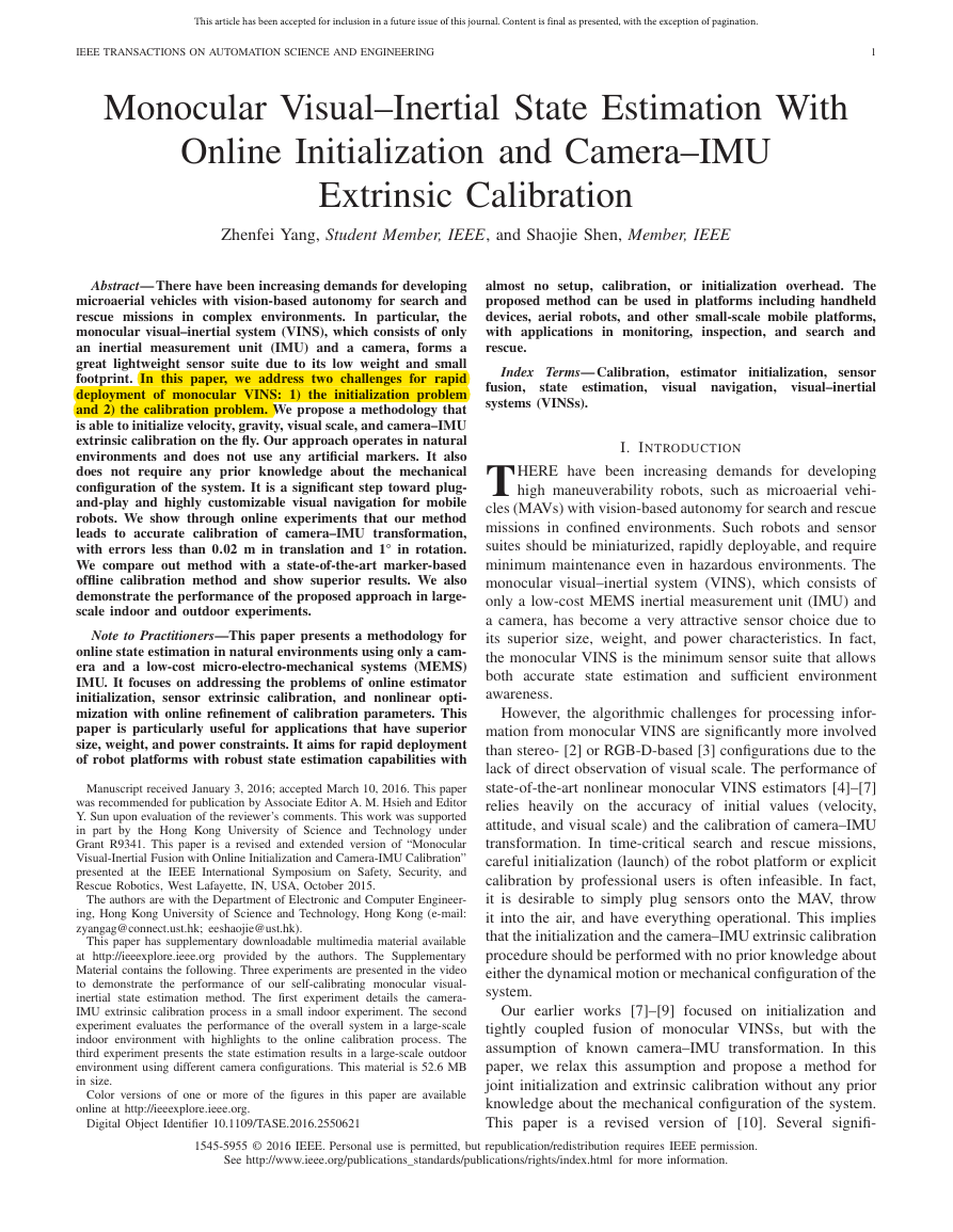
Fig. 1. Our monocular VINS setup with unknown camera–IMU extrinsic
calibration. Colored coordinate axes are plotted (red: x-axis, green: y-axis,
and blue: z-axis). Note that there are multiple 90° offsets between the camera
frame and the IMU frame. The rotation offsets are unknown to the estimator
and have to be calibrated online.
cant extensions have been made. First, we provide a more
thorough discussion of the full monocular VINS pipeline,
with additional details on the formulation of IMU preinte-
gration (Section IV) and nonlinear VINS with calibration
refinement (Section VI). Second, we compare our approach
against Kalibr, a state-of-the-art marker-based offline calibra-
tion method [1] (Section VIII-B) and show superior results.
We show through online experiments that our method leads to
accurate calibration of camera–IMU transformation with errors
of 0.02 m in translation and 1° in rotation. Finally, we present
large-scale outdoor experiments performed onboard a quadro-
tor aerial vehicle with different sensor placements and analyze
the results (Section VIII-D). Our approach is a substantial step
toward minimum sensing for plug-and-play robotic systems.
We identify the contributions of this paper as fourfold.
• A probabilistic optimization-based initialization proce-
dure that is able to recover all the essential navigation
quantities (initial velocity and attitude, visual scale,
and camera–IMU calibration) without any prior system
knowledge or artificial calibration objects.
• Principal criteria to identify convergence and termination
• A tightly coupled monocular visual–inertial
fusion
methodology for accurate state estimation with online
calibration refinement.
• Online experiments in complex indoor and outdoor
for the initialization procedure.
environments.
The rest of this paper is organized as follows. In Section II,
we discuss the relevant literature. We give an overview of the
complete system pipeline in Section III. In Section IV, we
present IMU preintegration, a core technique for summarizing
and utilizing high-rate IMU measurements without knowing
the initial attitude or velocity. We detail our linear initialization
and camera–IMU calibration procedure in Section V. A tightly
coupled, self-calibrating, nonlinear optimization-based monoc-
ular VINS estimator, which is built on top of [7] and [8], is
presented in Section VI. We present a two-way marginalization
scheme for handling of degenerate motions in Section VII
and discuss implementation details and present experimental
results in Section VIII. Finally, this paper is concluded with a
discussion of possible future research in Section IX.
�
This article has been accepted for inclusion in a future issue of this journal. Content is final as presented, with the exception of pagination.
YANG AND SHEN: MONOCULAR VISUAL–INERTIAL STATE ESTIMATION
3
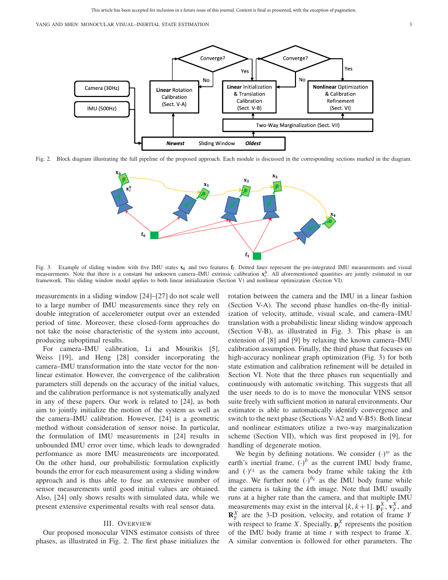
Fig. 2. Block diagram illustrating the full pipeline of the proposed approach. Each module is discussed in the corresponding sections marked in the diagram.
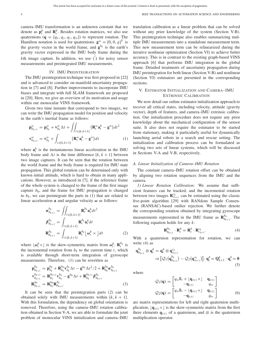
Fig. 3. Example of sliding window with five IMU states xk and two features fl. Dotted lines represent the pre-integrated IMU measurements and visual
measurements. Note that there is a constant but unknown camera–IMU extrinsic calibration xb
c . All aforementioned quantities are jointly estimated in our
framework. This sliding window model applies to both linear initialization (Section V) and nonlinear optimization (Section VI).
measurements in a sliding window [24]–[27] do not scale well
to a large number of IMU measurements since they rely on
double integration of accelerometer output over an extended
period of time. Moreover, these closed-form approaches do
not take the noise characteristic of the system into account,
producing suboptimal results.
and Mourikis
camera–IMU calibration, Li
[19], and Heng [28] consider
[5],
For
Weiss
incorporating the
camera–IMU transformation into the state vector for the non-
linear estimator. However, the convergence of the calibration
parameters still depends on the accuracy of the initial values,
and the calibration performance is not systematically analyzed
in any of these papers. Our work is related to [24], as both
aim to jointly initialize the motion of the system as well as
the camera–IMU calibration. However, [24] is a geometric
method without consideration of sensor noise. In particular,
the formulation of IMU measurements in [24] results in
unbounded IMU error over time, which leads to downgraded
performance as more IMU measurements are incorporated.
On the other hand, our probabilistic formulation explicitly
bounds the error for each measurement using a sliding window
approach and is thus able to fuse an extensive number of
sensor measurements until good initial values are obtained.
Also, [24] only shows results with simulated data, while we
present extensive experimental results with real sensor data.
III. OVERVIEW
Our proposed monocular VINS estimator consists of three
phases, as illustrated in Fig. 2. The first phase initializes the
rotation between the camera and the IMU in a linear fashion
(Section V-A). The second phase handles on-the-fly initial-
ization of velocity, attitude, visual scale, and camera–IMU
translation with a probabilistic linear sliding window approach
(Section V-B), as illustrated in Fig. 3. This phase is an
extension of [8] and [9] by relaxing the known camera–IMU
calibration assumption. Finally, the third phase that focuses on
high-accuracy nonlinear graph optimization (Fig. 3) for both
state estimation and calibration refinement will be detailed in
Section VI. Note that the three phases run sequentially and
continuously with automatic switching. This suggests that all
the user needs to do is to move the monocular VINS sensor
suite freely with sufficient motion in natural environments. Our
estimator is able to automatically identify convergence and
switch to the next phase (Sections V-A2 and V-B5). Both linear
and nonlinear estimators utilize a two-way marginalization
scheme (Section VII), which was first proposed in [9], for
handling of degenerate motion.
We begin by defining notations. We consider (·)w as the
earth’s inertial frame, (·)b as the current IMU body frame,
and (·)ck as the camera body frame while taking the kth
image. We further note (·)bk as the IMU body frame while
the camera is taking the kth image. Note that IMU usually
runs at a higher rate than the camera, and that multiple IMU
measurements may exist in the interval [k, k+1]. pX
Y , and
R X
Y are the 3-D position, velocity, and rotation of frame Y
with respect to frame X. Specially, pX
represents the position
t
of the IMU body frame at time t with respect to frame X.
A similar convention is followed for other parameters. The
Y , vX
�
This article has been accepted for inclusion in a future issue of this journal. Content is final as presented, with the exception of pagination.
4
IEEE TRANSACTIONS ON AUTOMATION SCIENCE AND ENGINEERING
c and Rb
camera–IMU transformation is an unknown constant that we
denote as pb
c . Besides rotation matrices, we also use
quaternions (q = [qx , qy, qz, qw]) to represent rotation. The
Hamilton notation is used for quaternions. gw = [0, 0, g]T is
the gravity vector in the world frame, and gbk is the earth’s
gravity vector expressed in the IMU body frame during the
kth image capture. In addition, we use ˆ(·) for noisy sensor
measurements and preintegrated IMU measurements.
IV. IMU PREINTEGRATION
The IMU preintegration technique was first proposed in [22]
and is advanced to consider on-manifold uncertainty propaga-
tion in [7] and [8]. Further improvements to incorporate IMU
biases and integrate with full SLAM framework are proposed
in [20]. Here, we give an overview of its motivation and usage
within our monocular VINS framework.
Given two time instants that correspond to two images, we
can write the IMU propagation model for position and velocity
in the earth’s inertial frame as follows:
�t +
pw
bk+1
vw
bk+1
bk
= pw
= vw
bk
bk
+ vw
+
t∈[k,k+1]
t∈[k,k+1]
− gw
Rw
t ab
t
Rw
t ab
t
dt
dt2
− gw
(1)
where ab
is the instantaneous linear acceleration in the IMU
body frame and �t is the time difference [k, k + 1] between
t
two image captures. It can be seen that the rotation between
the world frame and the body frame is required for IMU state
propagation. This global rotation can be determined only with
known initial attitude, which is hard to obtain in many appli-
cations. However, as introduced in [7], if the reference frame
of the whole system is changed to the frame of the first image
capture b0, and the frame for IMU propagation is changed
to bk, we can preintegrate the parts in (1) that are related to
linear acceleration a and angular velocity ω as follows:
=
=
=
αbk
bk+1
βbk
bk+1
Rbk
bk+1
t dt2
t∈[k,k+1] Rbk
t ab
t∈[k,k+1] Rbk
t ab
t∈[k,k+1] Rbk
ωb
t
t
t dt
×
dt
(2)
t
bk
t . Rbk
t
pb0
bk+1
vbk+1
bk+1
Rb0
bk+1
vbk
bk
− gb0�t + Rbk+1
× is the skew-symmetric matrix from ωb
where ωb
is
the incremental rotation from bk to the current time t, which
is available through short-term integration of gyroscope
measurements. Therefore, (1) can be rewritten as
�t − gb0�t2/2 + Rb0
+ Rb0
= pb0
bk
= Rbk+1
vbk
bk
= Rb0
Rbk
bk+1
It can be seen that
the preintegration parts (2) can be
obtained solely with IMU measurements within [k, k + 1].
With this formulation, the dependency on global orientation is
removed. Therefore, using the camera–IMU rotation calibra-
tion obtained in Section V-A, we are able to formulate the joint
problem of monocular VINS initialization and camera–IMU
bk+1
bk+1
βbk
αbk
(3)
bk
bk
bk
bk
.
translation calibration as a linear problem that can be solved
without any prior knowledge of the system (Section V-B).
This preintegration technique also enables summarizing mul-
tiple IMU measurements into a standalone measurement term.
This new measurement term can be relinearized during the
iterative nonlinear optimization (Section VI) to achieve better
accuracy. This is in contrast to the existing graph-based VINS
approach [6] that performs IMU integration in the global
frame. Detailed treatments of uncertainty propagation during
IMU preintegration for both linear (Section V-B) and nonlinear
(Section VI) estimators are presented in the corresponding
sections.
V. ESTIMATOR INITIALIZATION AND CAMERA–IMU
EXTRINSIC CALIBRATION
We now detail our online estimator initialization approach to
recover all critical states, including velocity, attitude (gravity
vector), depth of features, and camera–IMU extrinsic calibra-
tion. Our initialization procedure does not require any prior
knowledge about the mechanical configuration of the sensor
suite. It also does not require the estimator to be started
from stationary, making it particularly useful for dynamically
launching aerial robots in a search and rescue setting. The
initialization and calibration process can be formulated as
solving two sets of linear systems, which will be discussed
in Sections V-A and V-B, respectively.
A. Linear Initialization of Camera–IMU Rotation
The constant camera–IMU rotation offset can be obtained
by aligning two rotation sequences from the IMU and the
camera.
1) Linear Rotation Calibration: We assume that suffi-
cient features can be tracked, and the incremental rotation
between two images Rck
ck+1 can be estimated using the classic
five-point algorithm [29] with RANdom Sample Consen-
sus (RANSAC)-based outlier rejection. We further denote
the corresponding rotation obtained by integrating gyroscope
measurements represented in the IMU frame as Rbk
. The
following equation holds for any k:
= Rb
· Rb
bk+1
(4)
.
bk+1
Rbk
· Rck
ck+1
With a quaternion representation for
write (4) as
⊗ qb
qbk
bk+1
c
c
c
= qb
⇒Q1
⊗ qck
ck+1
qbk
bk+1
c
− Q2
qck
ck+1
· qb
c
rotation, we can
= Qk
k+1
· qb
c
= 0
(5)
where
Q1(q) =
Q2(q) =
qwI3 + qx yz×
qwI3 − qx yz×
−qx yz
−qx yz
qx yz
qw
qx yz
qw
(6)
are matrix representations for left and right quaternion multi-
plication, qx yz× is the skew-symmetric matrix from the first
three elements qx yz of a quaternion, and ⊗ is the quaternion
multiplication operator.
�
This article has been accepted for inclusion in a future issue of this journal. Content is final as presented, with the exception of pagination.
YANG AND SHEN: MONOCULAR VISUAL–INERTIAL STATE ESTIMATION
5
With multiple incremental rotations between pairs of con-
secutive images, we are able to construct the overconstrained
linear system as⎡
⎤
· qb
c
= QN · qb
c
= 0
(7)
⎢⎢⎢⎢⎢⎢⎣
w0
1
w1
2
⎥⎥⎥⎥⎥⎥⎦
2
1
· Q0
· Q1
...
· QN−1
N
wN−1
N
where N is the index of the latest frame that keeps grow-
ing until
the rotation calibration is completed. Note that
the incremental rotation measurements obtained from the
five-point algorithm contain outliers due to wrong correspon-
dences or numerical errors under degenerated motions. We use
k+1 derived from the robust norm for better outlier
weight wk
handling. As the rotation calibration runs with incoming mea-
surements, we are able to use the previously estimated camera–
c as the initial value to weight the residual
in a similar fashion to the Huber norm [30]. Specifically,
the residual is defined as the angle norm in the angle-axis
representation of the residual rotation matrix
IMU rotation ˆRb
− 1
/2
.
(8)
ˆRb
c Rck
The weight is a function of the residual
−1
−1
c Rbk
bk+1
k+1
r k
ck+1
ˆRb
= acos
tr
⎧⎨
⎩1,
=
k+1
wk
threshold
k+1
r k
k+1
r k
< threshold
, otherwise.
(9)
If
there are no sufficient
features for estimating the
camera rotation, wk
to zero. The solution to
the above linear system can be found as the right unit
singular vector corresponding to the smallest singular value
of QN .
is set
k+1
2) Termination Criteria: Successful calibration of
the
camera–IMU rotation Rb
c relies on sufficient rotation excita-
tion. Under sufficient rotation, the null space of QN should be
rank one. However, under degenerate motions in one or more
axes, the null space of QN may be larger than one. Therefore,
by checking whether the second smallest singular value of QN ,
σ min2
, is large enough, we have a good indicator of whether
R
sufficient rotation excitation is achieved. We set a singular
value threshold σR. The camera–IMU rotation calibration
process terminates if σ min2
> σR. A convergence plot can
be found in Fig. 6.
R
B. Linear Initialization of Velocity, Attitude, Feature Depth,
and Camera–IMU Translation
Once the camera–IMU rotation is fixed, we can estimate
the camera–IMU translation together with an initialization of
velocity, attitude, and feature depth, as well as the IMU poses
with respect to the initial reference frame, as in (3).
1) Linear Sliding Window Estimator: We use a tightly cou-
pled sliding window formulation (Fig. 3) for incorporating a
large number of IMU and camera measurements with constant
computational complexity. The initialization is done in the
IMU frame, with the full state vector defined as (the transpose
is ignored for simplicity of presentation)
xn, xn+1, . . . xn+N , pb
c
pb0
bk
, vbk
bk
, gbk
, λm , λm+1, . . . λm+M
(10)
X =
xk =
⎧⎨
⎩
minX
where xk is the kth IMU state, the gravity vector gbk deter-
mines the attitude (roll and pitch angles), N is the number
of IMU states in the sliding window, M is the number of
features that have sufficient parallax within the sliding window,
n and m are starting indexes of the sliding window, and
λl
is the depth of the lth feature from its first observation.
= [0, 0, 0] is preset. Note that we reuse the sensor
pb0
b0
measurements that we used for the camera–IMU rotation
calibration in this linear initialization phase, but with Rb
c fixed
as a constant. We also directly use the incremental (Rbk
) and
bk+1
relative (Rb0
) rotations obtained from short-term integration
of gyroscope measurements. As this linear initialization can
usually be done in only a few seconds, using the IMU rotation
directly will not cause significant drifts.
bk+1
The linear initialization is done with maximum likelihood
estimation by minimizing the sum of the Mahalanobis norm
of all measurement errors from the IMU and the monocular
camera within the sliding window
r p − H pX2 +
(l, j )∈C
ˆzc j
ˆzbk
k∈B
X2
− Hc j
+
l
bk+1
− Hbk
bk+1
⎫⎬
⎭
X2
Pbk
bk+1
l
bk+1
c j
λP
l
, Hc j
l
(11)
where B is the set of all IMU measurements, C is the set
of all observations between any features and any camera
poses, and Hbk
are corresponding measurement matri-
ces. {r p, H p} is the (optional) prior, which will be discussed
in Section V-B4. Since incremental and relative rotations are
known, (11) can be solved in a noniterative linear fashion.
2) Linear IMU Measurement Model: The linear IMU mea-
} between consecutive frames k and
surement {ˆzbk
bk+1
k + 1 is derived from (3), with the exception that all rotations
(Rb0
) are considered as known. We also introduce
bk
⎤
the propagation of body frame gravity vectors
⎥⎥⎦ = Hbk
ˆzk
k+1
, Hbk
bk+1
bk+1
X + nbk
bk+1
− vbk
− vbk
gbk+1 − gbk
bk
bk
�t + gbk
+ gbk �t
− pb0
bk
vbk+1
bk+1
Rbk
bk+1
bk+1
�t2
2
⎤
⎥⎥⎥⎦.
(12)
=
and Rbk
bk+1
⎡
ˆαbk
⎢⎢⎣
bk+1
ˆβ
bk
bk+1ˆ0
⎡
⎢⎢⎢⎣
Rbk
pb0
bk+1
b0
Rbk
=
The covariance Pbk
following form:
bk+1
Pbk
bk+1
of the linear IMU measurement has the
=
αβPbk
bk+1
0
0
gPbk
bk+1
.
(13)
�
This article has been accepted for inclusion in a future issue of this journal. Content is final as presented, with the exception of pagination.
6
IEEE TRANSACTIONS ON AUTOMATION SCIENCE AND ENGINEERING
k+1 is
Given known rotations, the joint covariance matrix αβPk
independent of the gravity covariance gPbk
bk+1. Consider the
continuous-time state-space model of the preintegrated IMU
measurements derived from the first two equations in (2)
˙αbk
t˙βbk
t
=
0
0
= Ft ·
+
αbk
0
t
Rbk
βbk
t
t
+ Gt · ab
.
t
I
0
αbk
t
βbk
t
ab
t
(14)
bk+1
αβPbk
can be calculated recursively using first-order discrete-
time propagation within the time interval [k, k+1] with initial
covariance Pbk
bk
αβPbk
t+δt
= (I + Ft δt) ·αβ Pbk
· (I + Ft δt)T
= 0
t
+ (Gt δt) · Qt · (Gt δt)T
(15)
where Qt is the covariance of the additive Gaussian noise of
the accelerometer measurements
ˆab
t
= ab
t
+ ant , ant ∼ N (0, Qt ).
(16)
l
, Hc j
l
3) Linear Camera Measurement Model: The linear camera
measurement model {ˆzc j
} for the observation of the lth
feature in the jth image is defined as
ˆzc j
⎛
⎜⎝λl
= ˆ0 = Hc j
X + λnc j
⎛
⎛
⎜⎝ f b0
⎜⎝ f b
−1
= M · f b
−1
0
b j
⎛
⎜⎝ f b
⎡
⎢⎣uci
⎞
⎞
⎟⎠
⎟⎠
⎞
⎞
⎟⎠
⎟⎠
⎤
⎥⎦
(17)
bi
c
c
l
l
l
l
vci
l
1
where M is defined as
M =
−1
0
0 −1
ˆuc j
ˆvc j
l
l
l
, vci
l
(18)
and [uci
] is the noiseless first observation of the lth feature
] is the observation
that happened in the ith image. [ˆuc j
of the same feature in the jth image. The function f m
(.) that
n
transforms a 3-D point r from frame n to frame m and its
inverse function f m
n
, ˆvc j
−1
l
l
(.) are defined as
(r) = Rm
· r + pm
·
r − pm
(r) = Rn
where all rotation matrices R X
f m
n
−1
f m
n
m
n
n
n
Y are known quantities.
λnc j
is the additive Gaussian measurement noise for the lin-
l
ear camera model, with the covariance matrix in the following
form:
λPc j
l
= λc j
2
l Pc j
l
(20)
where Pc j
is the feature observation noise in the normalized
l
image plane. Although we can only initialize the unknown λc j
l
as the average scene depth, we find in practice that the solution
is insensitive to the initial value of λc j
as long as it is set to
l
be larger than the actual depth.
(19)
4) Solution to the Linear Estimator: The linear cost func-
tion (11) can be rearranged into the following form:
(�p + �B + �C)X = (bp + bB + bC)
T H p, bp = H p
(21)
where {�B, bB} and {�C, bC} are information matrices and
vectors for IMU and visual measurements, respectively, and
T r p} is the (optional) prior. Due to
{�p = H p
the known incremental and relative rotations, the cost is linear
with respect to the states, and the system in (21) has a unique
solution, even the prior {� p, bp} is only used to lock the first
= [0, 0, 0]). This suggests that our method is
position (pb0
b0
able to recover all quantities in the full state vector, including
the camera–IMU translation, without any initial guess of those
values.
5) Termination Criteria: The covariance matrix (inverse of
� p + �B + �C
−1 naturally tells the
the information matrix)
uncertainty of the linear initialization estimator. The block that
corresponds to the camera–IMU translation in the covariance
matrix represents the uncertainty of the calibration parameters.
We use the maximum singular value σ max
of the block as the
convergence indicator and terminate the linear initialization
process if σ max
< σp, where σp is a threshold. A convergence
plot can be found in Fig. 6.
p
p
As computing the matrix inverse is much slower than
solving the linear system (29) using Cholesky decomposition,
we run the termination check at a slower rate in another thread.
This will slightly delay the termination time but will not harm
overall performance. After this point, the whole initialization
and calibration process is completed.
VI. TIGHTLY COUPLED NONLINEAR OPTIMIZATION
WITH CALIBRATION REFINEMENT
After state initialization and obtaining camera–IMU calibra-
tion (Section V), we proceed with a sliding window nonlinear
estimator, as illustrated in Fig. 3, for high-accuracy state
estimation and calibration refinement. This is an extension
of [7] and [8] by including camera–IMU calibration in the
nonlinear optimization.
Since a large number of parameters in the nonlinear opti-
mization share the same physical meaning as those in the linear
initialization (Section V), here we introduce a slight abuse of
notations by reusing symbols to represent state vectors (X ),
Jacobian matrices (H, F, G), covariance matrices (P, Q), and
information matrices (�).
A. Formulation
The definition of the full state is similar to the linear
case, with the exception that the full 6-DOF camera–IMU
transformation xb
c is included in the state vector. The gravity
vector is also replaced with the quaternion qbi
for joint
b j
optimization of IMU translation and rotation (the transpose
is again ignored)
X = [xn, xn+1,···x n+N , xb
xk =
=
, vbk
, qb0
pb0
bk
bk
bk
, qb
pb
.
c
c
xb
c
c
, λ0 ···λ m+M]
(22)
�
This article has been accepted for inclusion in a future issue of this journal. Content is final as presented, with the exception of pagination.
YANG AND SHEN: MONOCULAR VISUAL–INERTIAL STATE ESTIMATION
7
We minimize the sum of the Mahalanobis norm of all
measurement residuals to obtain a maximum a posteriori
estimation
minX
⎧⎨
rB
⎩r p − H pX2 +
k∈B
,X2
rC
ˆzc j
+
(l, j )∈C
,X ) and rC (ˆzc j
c j
P
l
l
bk+1
ˆzbk
⎫⎬
⎭
,X2
Pbk
bk+1
l
bk+1
where rB(ˆzbk
,X ) are measurement residuals
for the IMU and the camera, respectively. Corresponding
measurement models are defined in Sections VI-B and VI-C.
We use error-state representation [6] to linearize the nonlin-
ear system (23) and solve it with the Gauss–Newton algorithm
with the Huber norm [30] for robust outlier rejection. The
residuals for linear components such as position, velocity, and
feature depth can be easily defined as an addition to the latest
state estimates
p = ˆp + δp, v = ˆv + δv, λ = ˆλ + δλ.
(24)
The residual for rotation is instead modeled as the perturbation
in the tangent space of the rotation manifold. The error
quaternion term δq is defined as the small difference between
the estimated and the true quaternions
δq ≈
(25)
where ⊗ is the quaternion multiplication operator. The 3-D
error vector δθ is the minimal presentation of rotation residual.
We also have the equivalent formulation in the form of rotation
matrix to provide a simple linearization form for the rotation
residual
q = ˆq ⊗ δq,
δθ
1
1
2
R ≈ ˆR · (I + δθ×).
The full error-state vector then becomes
δX =
δxk =
=
δxb
c
, δλm . . . δλm+M
δxn, . . . δxn+N , δxb
c
, δvbk
δpb0
bk
bk
, δθ b
δpb
.
c
c
, δθ b0
bk
(26)
(27)
In each Gauss–Newton iteration, (23) is linearized at
current state estimation ˆX with respect to the error state δX
the
min
δX
⎧⎨
⎩r p − H pX2 +
ˆzc j
rC
(l, j )∈C
+
l
k∈B
rB
ˆzbk
, ˆX + Hbk
δX2
, ˆX + Hc j
bk+1
⎫⎬
⎭
l
c j
P
l
δX2
bk+1
Pbk
bk+1
(28)
bk+1
and Hc j
l
where Hbk
are Jacobians of IMU and visual
measurements, respectively. Minimizing the linearized cost
function (28) is equivalent to solving the following linear
system:
(� p + �B + �C)δX = (bp + bB + bC)
where � p, �B, and �C are information matrices from the
prior, IMU, and visual measurements, respectively. Incremen-
T r p} is
tal construction of the prior {�p = H p
discussed in Section VII. Note that (29) is different from (21)
in the sense that (29) solves for the increments for the
nonlinear optimization, while (21) directly recovers the initial
values.
T H p, bp = H p
(23)
The error state is updated as
ˆX = ˆX ⊕ δX
(30)
where ⊕ is the compound operator that has the form of simple
addition for position, velocity, and feature depth as in (24),
but is formulated as quaternion multiplication for rotations as
in (25).
B. IMU Measurement Model
ment is
Following (3), the residual of a preintegrated IMU measure-
⎡
⎢⎣δαbk
⎤
⎥⎦
2
bk
bk
x yz
rB
=
(31)
−1
0
bk
⎤
⎥⎥⎥⎦
,X =
�t − ˆαbk
bk+1
− ˆβ
bk
bk+1
− vbk
− vbk
⊗ qb0
bk+1
ˆzbk
bk+1
δβbk
bk+1
bk+1
δθ bk
⎡
bk+1
− pb0
+ gb0�t2/2
⎢⎢⎢⎣
Rbk
pb0
bk+1
b0
bk
+ gb0�t
vbk+1
Rbk
Rb0
ˆqb
bk+1
bk+1
b0
−1
⊗ qb
k
bk+1
where [q]x yz extracts the vector part of the quaternion q,
which forms the rotation error vector as in (25), and
]T is the preintegrated IMU measurement
[ˆαbk
bk+1
obtained following (2) without knowing the initial velocity
and attitude, using only noisy accelerometer and gyroscope
measurements
∼ N (0, Qt ).
(32)
Taking the derivative of the residual rB(ˆzbk
,X ) with
bk+1
respect to error-state vector δX gives the Jacobian of IMU
measurements Hbk
ant
ωnt
ˆab
tˆωb
−1
k
bk+1
in (28).
ant
ωnt
, ˆqb
ab
t
ωb
t
bk
bk+1
, ˆβ
=
+
,
t
t
bk+1
To obtain the covariance matrix Pbk
of the preintegrated
IMU measurement, we form the linearized continuous dynam-
ics of the error state of the IMU measurement using (2)
⎡
and (26)
δ˙αbk
⎢⎢⎣
δ ˙βbk
δ˙θ bk
⎡
⎢⎣δαbk
⎤
⎥⎥⎦ =
⎤
⎥⎦
t
δβbk
t
δθ bk
t
⎤
⎡
×
ˆab
⎥⎦
⎢⎣0
0− ˆRbk
−ˆωb
×
0
0
0
⎡
⎤
⎣ 0
⎦
0
− ˆRbk
ant
0
−I
ωnt
0
+
= Ft · δzbk
t + Gt · nt .
0
I
t
t
t
t
t
t
bk+1
(33)
(29)
The covariance matrix Pbk
can then be calculated by
first-order discrete-time propagation within the time interval
bk+1
�
ˆzc j
l
,X =
rC
=
f c j
l
⎤
l
− ˆu j
⎥⎥⎥⎥⎦
− ˆv j
⎤
⎥⎥⎦= f b
c
l
−1
⎡
⎢⎢⎢⎢⎣
⎡
⎢⎢⎣
f x c j
l
f zc j
l
f yc j
l
f zc j
l
f x c j
l
f yc j
l
f zc j
l
⎛
⎜⎝f b
−1
0
b j
⎛
⎜⎝f b0
bi
· f b
c
⎞
⎤
⎟⎠
⎥⎦
⎞
⎞
⎟⎠
⎟⎠
⎛
⎜⎝λl
⎡
⎢⎣uci
l
vci
l
1
(35)
This article has been accepted for inclusion in a future issue of this journal. Content is final as presented, with the exception of pagination.
8
IEEE TRANSACTIONS ON AUTOMATION SCIENCE AND ENGINEERING
[k, k + 1], with initial covariance Pbk
Pbk
t+δt
= (I+ Ft δt) · Pbk
bk
t
= 0
· (I+ Ft δt)T + (Gt δt) · Qt · (Gt δt)T .
(34)
Note how this propagation (33) is different from the dynamics
of the linear IMU model (14) as we also consider the error
propagation in the rotation component as well as the cross
correlation between the rotation and the translation.
C. Camera Measurement Model
The camera measurement model can be formulated similar
to the linear initialization (Section V-B), but with the residual
being the reprojection error with covariance matrix Pc j
l due to
the feature depth initialization presented in Section V-B
(.) and its inverse are defined in (19).
where f b
c
The Jacobian of the visual measurement Hc j
obtained by taking the derivative of the residual rC(ˆzc j
l
with respect to the error-state vector δX .
l
in (28) is
,X )
VII. TWO-WAY MARGINALIZATION
In order to bound the computational complexity of graph
optimization-based methods, marginalization is usually used.
We selectively marginalize out IMU states xk and features
λl from the sliding window for both the linear (Section V)
and nonlinear (Section VI) optimization. Due to the well-
known acceleration excitation requirement [13], [14] for scale
observability for monocular VINS, a naive strategy that always
marginalizes the oldest state may result in unobservable scale
in degenerate motions, such as hovering or constant velocity
motions.
To avoid this, we employ the two-way marginalization
scheme originally proposed in [8] and [9] to selectively remove
recent or old IMU states based on a scene parallax test. We add
a new IMU state to the sliding window if the time between
two IMU states �t is larger than a threshold. We do not have a
notion of spatial keyframes as in vision-only approaches [17],
due to the requirement of bounding the uncertainty for every
preintegrated IMU measurements. We then select whether to
remove the oldest or the most recent IMU states based on a
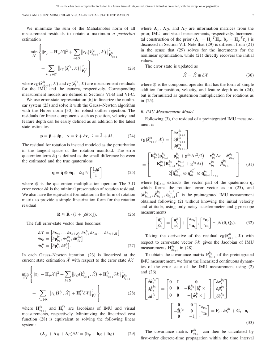
parallax test. As shown in Fig. 4, a recent state is identified
as fixed only if it has sufficient parallax to the previous fixed
state; otherwise, it will be removed in the next marginalization.
We refer readers to [9] for details of this selection process.
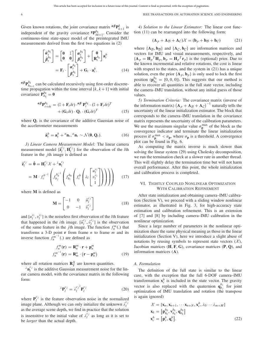
Fig. 4. Example with seven IMU states xk and three features fl . (a) Structure
of the full state before, during, and after marginalizing a recent IMU state x5
after a newer IMU state x6 is added. Visual and IMU measurements related
to IMU state x5 (denoted by transparent edges) are summarized into a new
prior �p in (36). Also, feature f2 is removed because it has no valid
observation (under the assumption that the first observation is noiseless, as
described in Section V-B3). (b) Similar marginalization process of the oldest
IMU state, where IMU state x0 and feature f0 are removed and all involved
measurements are used to construct a new prior. Small parallax: hovering or
slow motion in (a). Large parallax: fast motion in (b).
We construct a new prior based on all measurements related
to the removed states
� p = � p +
Hbk
Hc j
l Pc j
−1
l Hc j
−1
Pbk
bk+1
bk+1
Hbk
bk+1
+
l
(l, j )∈C−
k∈B−
and C−
where B−
are sets of removed IMU and camera
measurements, respectively. The marginalization is carried out
using the Schur complement [16].
(36)
Intuitively, the two-way marginalization keeps removing
recent IMU states if the platform has small or no motion.
Keeping older IMU states in this case will preserve accel-
eration information that is necessary to recover the visual
scale. The camera–IMU calibration also benefits from this
marginalization scheme because it naturally accumulates all
measurements to refine the calibration parameters.
VIII. EXPERIMENTAL RESULTS
A. Implementation Details
As shown in Fig. 1, our monocular VINS sensor suite
consists of an mvBlueFOX-MLC200w grayscale camera with
�




 2023年江西萍乡中考道德与法治真题及答案.doc
 2012年重庆南川中考生物真题及答案.doc
 2013年江西师范大学地理学综合及文艺理论基础考研真题.doc
 2020年四川甘孜小升初语文真题及答案I卷.doc
 2020年注册岩土工程师专业基础考试真题及答案.doc
 2023-2024学年福建省厦门市九年级上学期数学月考试题及答案.doc
 2021-2022学年辽宁省沈阳市大东区九年级上学期语文期末试题及答案.doc
 2022-2023学年北京东城区初三第一学期物理期末试卷及答案.doc
 2018上半年江西教师资格初中地理学科知识与教学能力真题及答案.doc
 2012年河北国家公务员申论考试真题及答案-省级.doc
 2020-2021学年江苏省扬州市江都区邵樊片九年级上学期数学第一次质量检测试题及答案.doc
 2022下半年黑龙江教师资格证中学综合素质真题及答案.doc