Experimental Modal Analysis
A Simple Non-Mathematical Presentation
Peter Avitabile, University of Massachusetts Lowell, Lowell, Massachusetts
Often times, people ask some simple questions regarding
modal analysis and how structures vibrate. Most times, it is
impossible to describe this simply and some of the basic un-
derlying theory needs to be addressed in order to fully explain
some of these concepts. However, many times the theory is just
a little too much to handle and some of the concepts can be
described without a rigorous mathematical treatment. This
article will attempt to explain some concepts about how struc-
tures vibrate and the use of some of the tools to solve struc-
tural dynamic problems. The intent of this article is to sim-
ply identify how structures vibrate from a nonmathematical
perspective. With this being said, let’s start with the first ques-
tion that is usually asked:
Could you explain modal analysis for me?
In a nutshell, we could say that modal analysis is a process
whereby we describe a structure in terms of its natural char-
acteristics which are the frequency, damping and mode shapes
– its dynamic properties. Well that’s a mouthful so let’s explain
what that means. Without getting too technical, I often explain
modal analysis in terms of the modes of vibration of a simple
plate. This explanation is usually useful for engineers who are
new to vibrations and modal analysis.
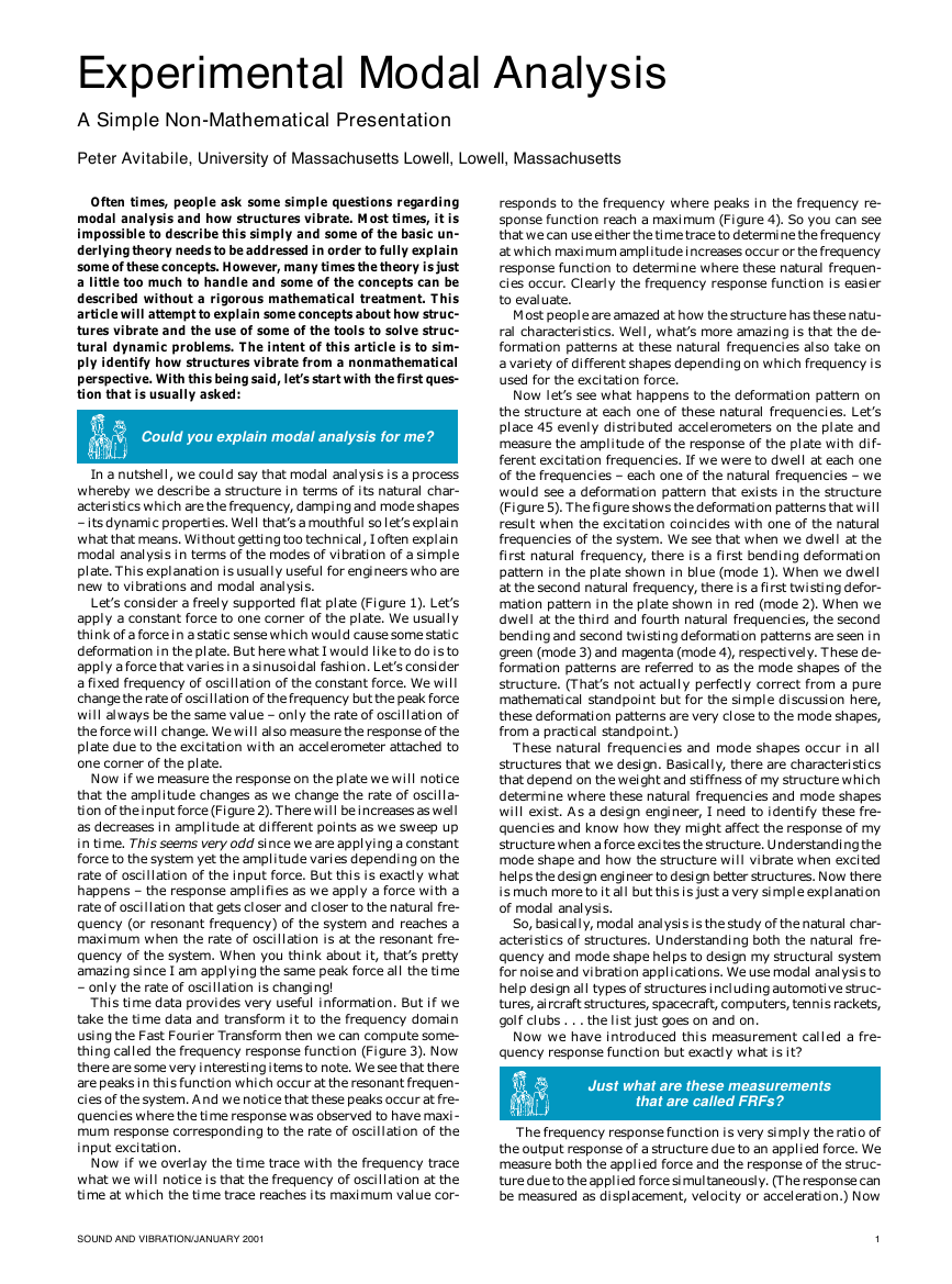
Let’s consider a freely supported flat plate (Figure 1). Let’s
apply a constant force to one corner of the plate. We usually
think of a force in a static sense which would cause some static
deformation in the plate. But here what I would like to do is to
apply a force that varies in a sinusoidal fashion. Let’s consider
a fixed frequency of oscillation of the constant force. We will
change the rate of oscillation of the frequency but the peak force
will always be the same value – only the rate of oscillation of
the force will change. We will also measure the response of the
plate due to the excitation with an accelerometer attached to
one corner of the plate.
Now if we measure the response on the plate we will notice
that the amplitude changes as we change the rate of oscilla-
tion of the input force (Figure 2). There will be increases as well
as decreases in amplitude at different points as we sweep up
in time. This seems very odd since we are applying a constant
force to the system yet the amplitude varies depending on the
rate of oscillation of the input force. But this is exactly what
happens – the response amplifies as we apply a force with a
rate of oscillation that gets closer and closer to the natural fre-
quency (or resonant frequency) of the system and reaches a
maximum when the rate of oscillation is at the resonant fre-
quency of the system. When you think about it, that’s pretty
amazing since I am applying the same peak force all the time
– only the rate of oscillation is changing!
This time data provides very useful information. But if we
take the time data and transform it to the frequency domain
using the Fast Fourier Transform then we can compute some-
thing called the frequency response function (Figure 3). Now
there are some very interesting items to note. We see that there
are peaks in this function which occur at the resonant frequen-
cies of the system. And we notice that these peaks occur at fre-
quencies where the time response was observed to have maxi-
mum response corresponding to the rate of oscillation of the
input excitation.
Now if we overlay the time trace with the frequency trace
what we will notice is that the frequency of oscillation at the
time at which the time trace reaches its maximum value cor-
responds to the frequency where peaks in the frequency re-
sponse function reach a maximum (Figure 4). So you can see
that we can use either the time trace to determine the frequency
at which maximum amplitude increases occur or the frequency
response function to determine where these natural frequen-
cies occur. Clearly the frequency response function is easier
to evaluate.
Most people are amazed at how the structure has these natu-
ral characteristics. Well, what’s more amazing is that the de-
formation patterns at these natural frequencies also take on
a variety of different shapes depending on which frequency is
used for the excitation force.
Now let’s see what happens to the deformation pattern on
the structure at each one of these natural frequencies. Let’s
place 45 evenly distributed accelerometers on the plate and
measure the amplitude of the response of the plate with dif-
ferent excitation frequencies. If we were to dwell at each one
of the frequencies – each one of the natural frequencies – we
would see a deformation pattern that exists in the structure
(Figure 5). The figure shows the deformation patterns that will
result when the excitation coincides with one of the natural
frequencies of the system. We see that when we dwell at the
first natural frequency, there is a first bending deformation
pattern in the plate shown in blue (mode 1). When we dwell
at the second natural frequency, there is a first twisting defor-
mation pattern in the plate shown in red (mode 2). When we
dwell at the third and fourth natural frequencies, the second
bending and second twisting deformation patterns are seen in
green (mode 3) and magenta (mode 4), respectively. These de-
formation patterns are referred to as the mode shapes of the
structure. (That’s not actually perfectly correct from a pure
mathematical standpoint but for the simple discussion here,
these deformation patterns are very close to the mode shapes,
from a practical standpoint.)
These natural frequencies and mode shapes occur in all
structures that we design. Basically, there are characteristics
that depend on the weight and stiffness of my structure which
determine where these natural frequencies and mode shapes
will exist. As a design engineer, I need to identify these fre-
quencies and know how they might affect the response of my
structure when a force excites the structure. Understanding the
mode shape and how the structure will vibrate when excited
helps the design engineer to design better structures. Now there
is much more to it all but this is just a very simple explanation
of modal analysis.
So, basically, modal analysis is the study of the natural char-
acteristics of structures. Understanding both the natural fre-
quency and mode shape helps to design my structural system
for noise and vibration applications. We use modal analysis to
help design all types of structures including automotive struc-
tures, aircraft structures, spacecraft, computers, tennis rackets,
golf clubs . . . the list just goes on and on.
Now we have introduced this measurement called a fre-
quency response function but exactly what is it?
Just what are these measurements
that are called FRFs?
The frequency response function is very simply the ratio of
the output response of a structure due to an applied force. We
measure both the applied force and the response of the struc-
ture due to the applied force simultaneously. (The response can
be measured as displacement, velocity or acceleration.) Now
SOUND AND VIBRATION/JANUARY 2001
1
�
Output Response
Input Force
1
2
3
Figure 1. Simple plate excitation/response model.
Increasing Rate of Oscillation
Figure 2. Simple plate response.
e
d
u
t
i
n
g
a
M
Figure 3. Simple plate frequency response function.
Frequency
Figure 4. Overlay of time and frequency response functions.
Mode 1
Mode 3
Mode 2
Mode 4
Figure 5. Simple plate sine dwell responses.
8
5
2
8
0
−3
8
7
−6
Figure 6. A 3 DOF model of a beam.
the measured time data is transformed from the time domain
to the frequency domain using a Fast Fourier Transform algo-
rithm found in any signal processing analyzer and computer
software packages.
Due to this transformation, the functions end up being com-
plex valued numbers; the functions contain real and imaginary
components or magnitude and phase components to describe
the function. So let’s take a look at what some of the functions
might look like and try to determine how modal data can be
extracted from these measured functions.
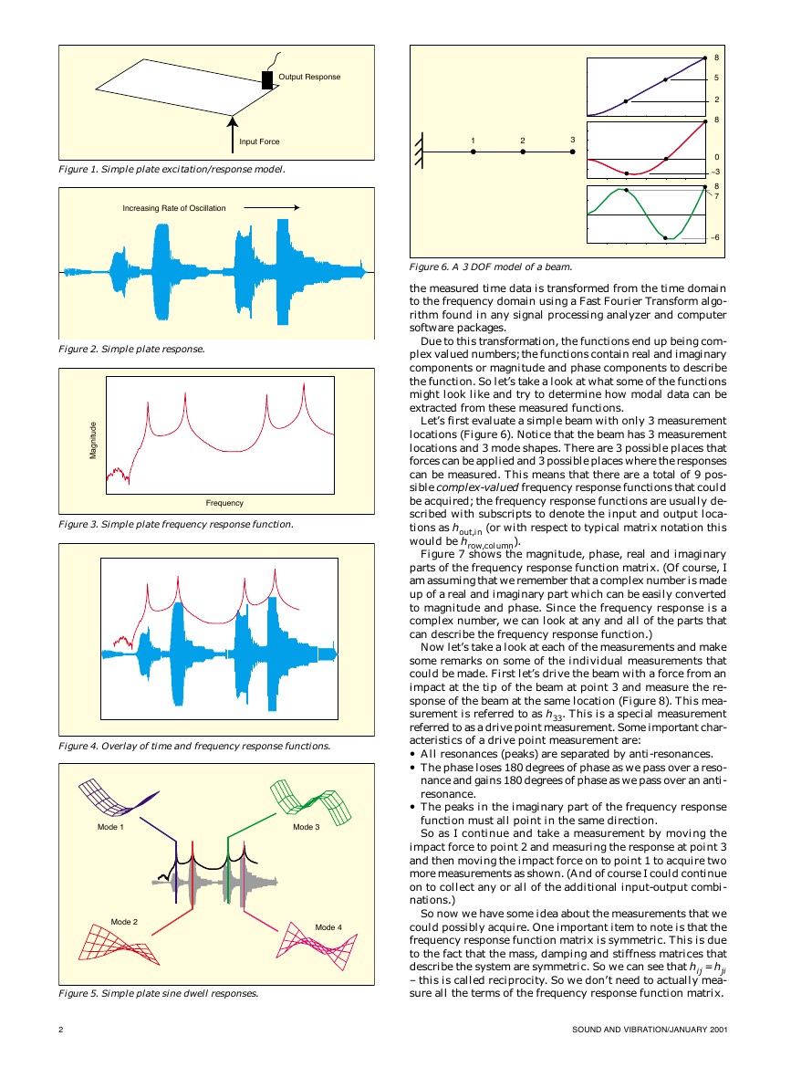
Let’s first evaluate a simple beam with only 3 measurement
locations (Figure 6). Notice that the beam has 3 measurement
locations and 3 mode shapes. There are 3 possible places that
forces can be applied and 3 possible places where the responses
can be measured. This means that there are a total of 9 pos-
sible complex-valued frequency response functions that could
be acquired; the frequency response functions are usually de-
scribed with subscripts to denote the input and output loca-
tions as hout,in (or with respect to typical matrix notation this
would be hrow,column).
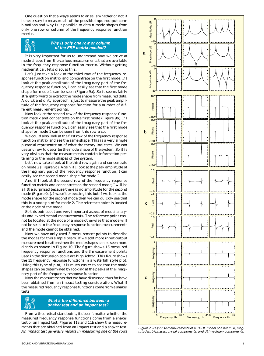
Figure 7 shows the magnitude, phase, real and imaginary
parts of the frequency response function matrix. (Of course, I
am assuming that we remember that a complex number is made
up of a real and imaginary part which can be easily converted
to magnitude and phase. Since the frequency response is a
complex number, we can look at any and all of the parts that
can describe the frequency response function.)
Now let’s take a look at each of the measurements and make
some remarks on some of the individual measurements that
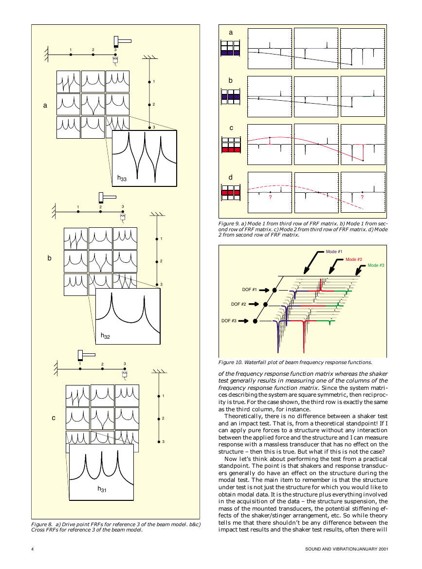
could be made. First let’s drive the beam with a force from an
impact at the tip of the beam at point 3 and measure the re-
sponse of the beam at the same location (Figure 8). This mea-
surement is referred to as h33. This is a special measurement
referred to as a drive point measurement. Some important char-
acteristics of a drive point measurement are:
a All resonances (peaks) are separated by anti-resonances.
a The phase loses 180 degrees of phase as we pass over a reso-
nance and gains 180 degrees of phase as we pass over an anti-
resonance.
a The peaks in the imaginary part of the frequency response
function must all point in the same direction.
So as I continue and take a measurement by moving the
impact force to point 2 and measuring the response at point 3
and then moving the impact force on to point 1 to acquire two
more measurements as shown. (And of course I could continue
on to collect any or all of the additional input-output combi-
nations.)
So now we have some idea about the measurements that we
could possibly acquire. One important item to note is that the
frequency response function matrix is symmetric. This is due
to the fact that the mass, damping and stiffness matrices that
describe the system are symmetric. So we can see that hij = hji
– this is called reciprocity. So we don’t need to actually mea-
sure all the terms of the frequency response function matrix.
2
SOUND AND VIBRATION/JANUARY 2001
�
One question that always seems to arise is whether or not it
is necessary to measure all of the possible input-output com-
binations and why is it possible to obtain mode shapes from
only one row or column of the frequency response function
matrix.
Why is only one row or column
of the FRF matrix needed?
It is very important for us to understand how we arrive at
mode shapes from the various measurements that are available
in the frequency response function matrix. Without getting
mathematical, let’s discuss this.
Let’s just take a look at the third row of the frequency re-
sponse function matrix and concentrate on the first mode. If I
look at the peak amplitude of the imaginary part of the fre-
quency response function, I can easily see that the first mode
shape for mode 1 can be seen (Figure 9a). So it seems fairly
straightforward to extract the mode shape from measured data.
A quick and dirty approach is just to measure the peak ampli-
tude of the frequency response function for a number of dif-
ferent measurement points.
Now look at the second row of the frequency response func-
tion matrix and concentrate on the first mode (Figure 9b). If I
look at the peak amplitude of the imaginary part of the fre-
quency response function, I can easily see that the first mode
shape for mode 1 can be seen from this row also.
We could also look at the first row of the frequency response
function matrix and see the same shape. This is a very simple
pictorial representation of what the theory indicates. We can
use any row to describe the mode shape of the system. So it is
very obvious that the measurements contain information per-
taining to the mode shapes of the system.
Let’s now take a look at the third row again and concentrate
on mode 2 (Figure 9c). Again if I look at the peak amplitude of
the imaginary part of the frequency response function, I can
easily see the second mode shape for mode 2.
And if I look at the second row of the frequency response
function matrix and concentrate on the second mode, I will be
a little surprised because there is no amplitude for the second
mode (Figure 9d). I wasn’t expecting this but if we look at the
mode shape for the second mode then we can quickly see that
this is a node point for mode 2. The reference point is located
at the node of the mode.
So this points out one very important aspect of modal analy-
sis and experimental measurements. The reference point can-
not be located at the node of a mode otherwise that mode will
not be seen in the frequency response function measurements
and the mode cannot be obtained.
Now we have only used 3 measurement points to describe
the modes for this simple beam. If we add more input-output
measurement locations then the mode shapes can be seen more
clearly as shown in Figure 10. The figure shows 15 measured
frequency response functions and the 3 measurement points
used in the discussion above are highlighted. This figure shows
the 15 frequency response functions in a waterfall style plot.
Using this type of plot, it is much easier to see that the mode
shapes can be determined by looking at the peaks of the imagi-
nary part of the frequency response function.
Now the measurements that we have discussed thus far have
been obtained from an impact testing consideration. What if
the measured frequency response functions come from a shaker
test?
What’s the difference between a
shaker test and an impact test?
From a theoretical standpoint, it doesn’t matter whether the
measured frequency response functions come from a shaker
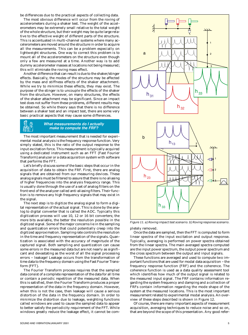
test or an impact test. Figures 11a and 11b show the measure-
ments that are obtained from an impact test and a shaker test.
An impact test generally results in measuring one of the rows
a
0
B
d
,
e
d
u
t
i
n
g
a
M
−80
0
B
d
,
e
d
u
t
i
n
g
a
M
−80
0
B
d
,
e
d
u
t
i
n
g
a
M
−80
180˚
e
s
a
h
P
−180˚
180˚
b
e
s
a
h
P
−180˚
180˚
e
s
a
h
P
−180˚
0.5
l
a
e
R
−0.5
0.5
c
l
a
e
R
−0.5
0.5
l
a
e
R
−0.5
d
1
y
r
a
n
g
a
m
i
I
−1
1
y
r
a
n
g
a
m
i
I
−1
1
y
r
a
n
g
a
m
i
I
−1
0
Frequency, Hz
40
0
Frequency, Hz
40
0
Frequency, Hz
40
Figure 7. Response measurements of a 3 DOF model of a beam: a) mag-
nitudes; b) phases; c) real components; and d) imaginary components.
SOUND AND VIBRATION/JANUARY 2001
3
�
a
b
c
1
2
3
h33
1
2
3
h32
1
2
3
h31
1
2
3
1
2
3
1
2
3
Figure 8. a) Drive point FRFs for reference 3 of the beam model. b&c)
Cross FRFs for reference 3 of the beam model.
a
b
c
d
?
?
Figure 9. a) Mode 1 from third row of FRF matrix. b) Mode 1 from sec-
ond row of FRF matrix. c) Mode 2 from third row of FRF matrix. d) Mode
2 from second row of FRF matrix.
Mode #1
Mode #2
Mode #3
DOF #1
DOF #2
DOF #3
Figure 10. Waterfall plot of beam frequency response functions.
of the frequency response function matrix whereas the shaker
test generally results in measuring one of the columns of the
frequency response function matrix. Since the system matri-
ces describing the system are square symmetric, then reciproc-
ity is true. For the case shown, the third row is exactly the same
as the third column, for instance.
Theoretically, there is no difference between a shaker test
and an impact test. That is, from a theoretical standpoint! If I
can apply pure forces to a structure without any interaction
between the applied force and the structure and I can measure
response with a massless transducer that has no effect on the
structure – then this is true. But what if this is not the case?
Now let’s think about performing the test from a practical
standpoint. The point is that shakers and response transduc-
ers generally do have an effect on the structure during the
modal test. The main item to remember is that the structure
under test is not just the structure for which you would like to
obtain modal data. It is the structure plus everything involved
in the acquisition of the data – the structure suspension, the
mass of the mounted transducers, the potential stiffening ef-
fects of the shaker/stinger arrangement, etc. So while theory
tells me that there shouldn’t be any difference between the
impact test results and the shaker test results, often there will
4
SOUND AND VIBRATION/JANUARY 2001
�
be differences due to the practical aspects of collecting data.
The most obvious difference will occur from the roving of
accelerometers during a shaker test. The weight of the accel-
erometers may be extremely small relative to the total weight
of the whole structure, but their weight may be quite large rela-
tive to the effective weight of different parts of the structure.
This is accentuated in multi-channel systems where many ac-
celerometers are moved around the structure in order to acquire
all the measurements. This can be a problem especially on
lightweight structures. One way to correct this problem is to
mount all of the accelerometers on the structure even though
only a few are measured at a time. Another way is to add
dummy accelerometer masses at locations not being measured;
this will eliminate the roving mass effect.
Another difference that can result is due to the shaker/stinger
effects. Basically, the modes of the structure may be affected
by the mass and stiffness effects of the shaker attachment.
While we try to minimize these effects, they may exist. The
purpose of the stinger is to uncouple the effects of the shaker
from the structure. However, on many structures, the effects
of the shaker attachment may be significant. Since an impact
test does not suffer from these problems, different results may
be obtained. So while theory says that there is no difference
between a shaker test and an impact test, there are some very
basic practical aspects that may cause some differences.
What measurements do I actually
make to compute the FRF?
The most important measurement that is needed for experi-
mental modal analysis is the frequency response function. Very
simply stated, this is the ratio of the output response to the
input excitation force. This measurement is typically acquired
using a dedicated instrument such as an FFT (Fast Fourier
Transform) analyzer or a data acquisition system with software
that performs the FFT.
Let’s briefly discuss some of the basic steps that occur in the
acquisition of data to obtain the FRF. First, there are analog
signals that are obtained from our measuring devices. These
analog signals must be filtered to assure that there is no aliasing
of higher frequencies into the analysis frequency range. This
is usually done through the use of a set of analog filters on the
front-end of the analyzer called anti-aliasing filters. Their func-
tion is to remove any high frequency signals that may exist in
the signal.
The next step is to digitize the analog signal to form a digi-
tal representation of the actual signal. This is done by the ana-
log to digital converter that is called the ADC. Typically this
digitization process will use 10, 12 or 16 bit converters; the
more bits available, the better the resolution possible in the
digitized signal. Some of the major concerns lie in the sampling
and quantization errors that could potentially creep into the
digitized approximation. Sampling rate controls the resolution
in the time and frequency representation of the signals. Quan-
tization is associated with the accuracy of magnitude of the
captured signal. Both sampling and quantization can cause
some errors in the measured data but are not nearly as signifi-
cant and devastating as the worst of all the signal processing
errors – leakage! Leakage occurs from the transformation of
time data to the frequency domain using the Fast Fourier Trans-
form (FFT).
The Fourier Transform process requires that the sampled
data consist of a complete representation of the data for all time
or contain a periodic repetition of the measured data. When
this is satisfied, then the Fourier Transform produces a proper
representation of the data in the frequency domain. However,
when this is not the case, then leakage will cause a serious
distortion of the data in the frequency domain. In order to
minimize the distortion due to leakage, weighting functions
called windows are used to cause the sampled data to appear
to better satisfy the periodicity requirement of the FFT. While
windows greatly reduce the leakage effect, it cannot be com-
1
2
3
a
b
h 31
h 33
h 32
h13
3
h 23
h 33
1
2
3
1
2
3
Figure 11. a) Roving impact test scenario. b) Roving response scenario.
pletely removed.
Once the data are sampled, then the FFT is computed to form
linear spectra of the input excitation and output response.
Typically, averaging is performed on power spectra obtained
from the linear spectra. The main averaged spectra computed
are the input power spectrum, the output power spectrum and
the cross spectrum between the output and input signals.
These functions are averaged and used to compute two im-
portant functions that are used for modal data acquisition – the
frequency response function (FRF) and the coherence. The
coherence function is used as a data quality assessment tool
which identifies how much of the output signal is related to
the measured input signal. The FRF contains information re-
garding the system frequency and damping and a collection of
FRFs contain information regarding the mode shape of the
system at the measured locations. This is the most important
measurement related to experimental modal analysis. An over-
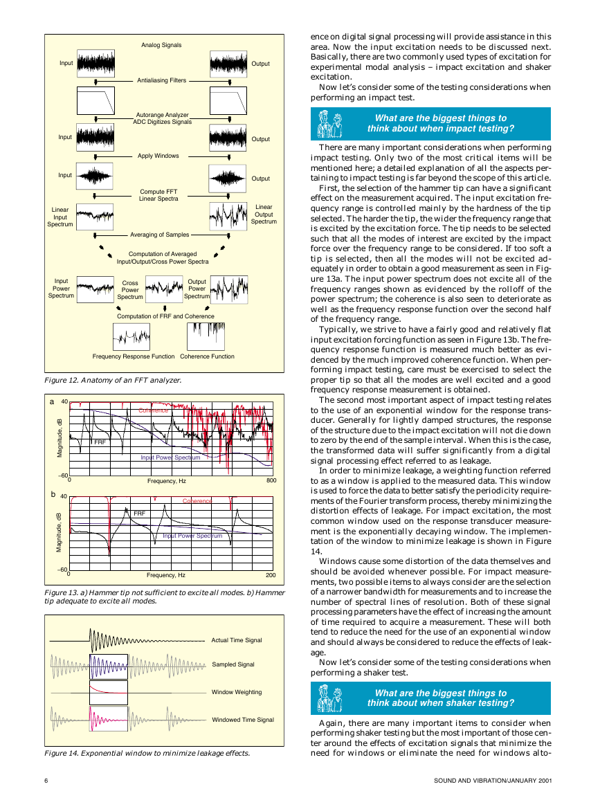
view of these steps described is shown in Figure 12.
Of course, there are many important aspects of measurement
acquisition, averaging techniques to reduce noise and so on,
that are beyond the scope of this presentation. Any good refer-
SOUND AND VIBRATION/JANUARY 2001
5
�
Input
Input
Input
Linear
Input
Spectrum
Analog Signals
Antialiasing Filters
Autorange Analyzer
ADC Digitizes Signals
Apply Windows
Compute FFT
Linear Spectra
Output
Output
Output
Linear
Output
Spectrum
Averaging of Samples
Computation of Averaged
Input/Output/Cross Power Spectra
Input
Power
Spectrum
Cross
Power
Spectrum
Output
Power
Spectrum
Computation of FRF and Coherence
Frequency Response Function Coherence Function
Figure 12. Anatomy of an FFT analyzer.
a
40
B
d
,
e
d
u
t
i
n
g
a
M
−60
0
b
40
B
d
,
e
d
u
t
i
n
g
a
M
−60
0
Coherence
FRF
Input Power Spectrum
Frequency, Hz
800
Coherence
FRF
Input Power Spectrum
Frequency, Hz
200
Figure 13. a) Hammer tip not sufficient to excite all modes. b) Hammer
tip adequate to excite all modes.
Actual Time Signal
Sampled Signal
Window Weighting
Windowed Time Signal
Figure 14. Exponential window to minimize leakage effects.
ence on digital signal processing will provide assistance in this
area. Now the input excitation needs to be discussed next.
Basically, there are two commonly used types of excitation for
experimental modal analysis – impact excitation and shaker
excitation.
Now let’s consider some of the testing considerations when
performing an impact test.
What are the biggest things to
think about when impact testing?
There are many important considerations when performing
impact testing. Only two of the most critical items will be
mentioned here; a detailed explanation of all the aspects per-
taining to impact testing is far beyond the scope of this article.
First, the selection of the hammer tip can have a significant
effect on the measurement acquired. The input excitation fre-
quency range is controlled mainly by the hardness of the tip
selected. The harder the tip, the wider the frequency range that
is excited by the excitation force. The tip needs to be selected
such that all the modes of interest are excited by the impact
force over the frequency range to be considered. If too soft a
tip is selected, then all the modes will not be excited ad-
equately in order to obtain a good measurement as seen in Fig-
ure 13a. The input power spectrum does not excite all of the
frequency ranges shown as evidenced by the rolloff of the
power spectrum; the coherence is also seen to deteriorate as
well as the frequency response function over the second half
of the frequency range.
Typically, we strive to have a fairly good and relatively flat
input excitation forcing function as seen in Figure 13b. The fre-
quency response function is measured much better as evi-
denced by the much improved coherence function. When per-
forming impact testing, care must be exercised to select the
proper tip so that all the modes are well excited and a good
frequency response measurement is obtained.
The second most important aspect of impact testing relates
to the use of an exponential window for the response trans-
ducer. Generally for lightly damped structures, the response
of the structure due to the impact excitation will not die down
to zero by the end of the sample interval. When this is the case,
the transformed data will suffer significantly from a digital
signal processing effect referred to as leakage.
In order to minimize leakage, a weighting function referred
to as a window is applied to the measured data. This window
is used to force the data to better satisfy the periodicity require-
ments of the Fourier transform process, thereby minimizing the
distortion effects of leakage. For impact excitation, the most
common window used on the response transducer measure-
ment is the exponentially decaying window. The implemen-
tation of the window to minimize leakage is shown in Figure
14.
Windows cause some distortion of the data themselves and
should be avoided whenever possible. For impact measure-
ments, two possible items to always consider are the selection
of a narrower bandwidth for measurements and to increase the
number of spectral lines of resolution. Both of these signal
processing parameters have the effect of increasing the amount
of time required to acquire a measurement. These will both
tend to reduce the need for the use of an exponential window
and should always be considered to reduce the effects of leak-
age.
Now let’s consider some of the testing considerations when
performing a shaker test.
What are the biggest things to
think about when shaker testing?
Again, there are many important items to consider when
performing shaker testing but the most important of those cen-
ter around the effects of excitation signals that minimize the
need for windows or eliminate the need for windows alto-
6
SOUND AND VIBRATION/JANUARY 2001
�
gether. There are many other considerations when performing
shaker testing but a detailed explanation of all of these is far
beyond the scope of this presentation.
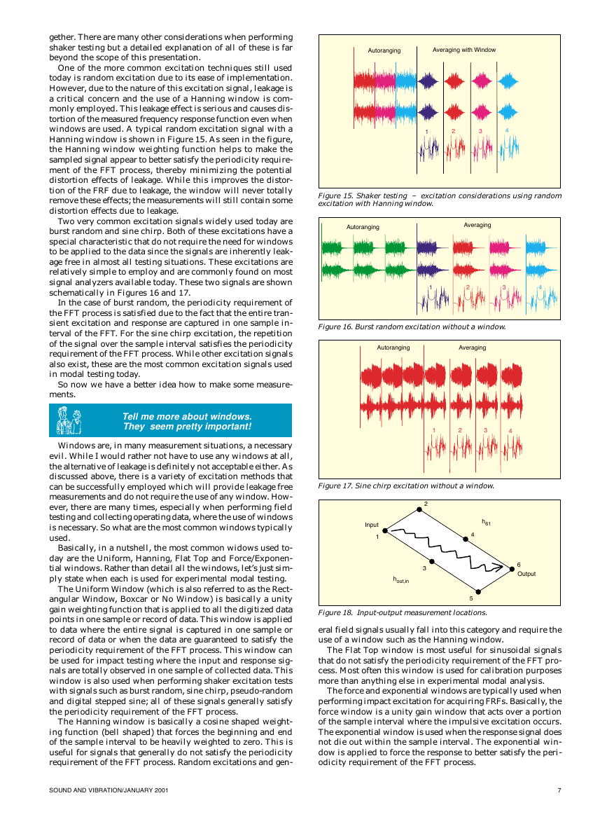
One of the more common excitation techniques still used
today is random excitation due to its ease of implementation.
However, due to the nature of this excitation signal, leakage is
a critical concern and the use of a Hanning window is com-
monly employed. This leakage effect is serious and causes dis-
tortion of the measured frequency response function even when
windows are used. A typical random excitation signal with a
Hanning window is shown in Figure 15. As seen in the figure,
the Hanning window weighting function helps to make the
sampled signal appear to better satisfy the periodicity require-
ment of the FFT process, thereby minimizing the potential
distortion effects of leakage. While this improves the distor-
tion of the FRF due to leakage, the window will never totally
remove these effects; the measurements will still contain some
distortion effects due to leakage.
Two very common excitation signals widely used today are
burst random and sine chirp. Both of these excitations have a
special characteristic that do not require the need for windows
to be applied to the data since the signals are inherently leak-
age free in almost all testing situations. These excitations are
relatively simple to employ and are commonly found on most
signal analyzers available today. These two signals are shown
schematically in Figures 16 and 17.
In the case of burst random, the periodicity requirement of
the FFT process is satisfied due to the fact that the entire tran-
sient excitation and response are captured in one sample in-
terval of the FFT. For the sine chirp excitation, the repetition
of the signal over the sample interval satisfies the periodicity
requirement of the FFT process. While other excitation signals
also exist, these are the most common excitation signals used
in modal testing today.
So now we have a better idea how to make some measure-
ments.
Tell me more about windows.
They seem pretty important!
Windows are, in many measurement situations, a necessary
evil. While I would rather not have to use any windows at all,
the alternative of leakage is definitely not acceptable either. As
discussed above, there is a variety of excitation methods that
can be successfully employed which will provide leakage free
measurements and do not require the use of any window. How-
ever, there are many times, especially when performing field
testing and collecting operating data, where the use of windows
is necessary. So what are the most common windows typically
used.
Basically, in a nutshell, the most common widows used to-
day are the Uniform, Hanning, Flat Top and Force/Exponen-
tial windows. Rather than detail all the windows, let’s just sim-
ply state when each is used for experimental modal testing.
The Uniform Window (which is also referred to as the Rect-
angular Window, Boxcar or No Window) is basically a unity
gain weighting function that is applied to all the digitized data
points in one sample or record of data. This window is applied
to data where the entire signal is captured in one sample or
record of data or when the data are guaranteed to satisfy the
periodicity requirement of the FFT process. This window can
be used for impact testing where the input and response sig-
nals are totally observed in one sample of collected data. This
window is also used when performing shaker excitation tests
with signals such as burst random, sine chirp, pseudo-random
and digital stepped sine; all of these signals generally satisfy
the periodicity requirement of the FFT process.
The Hanning window is basically a cosine shaped weight-
ing function (bell shaped) that forces the beginning and end
of the sample interval to be heavily weighted to zero. This is
useful for signals that generally do not satisfy the periodicity
requirement of the FFT process. Random excitations and gen-
Autoranging
Averaging with Window
1
2
3
4
Figure 15. Shaker testing – excitation considerations using random
excitation with Hanning window.
Autoranging
Averaging
1
2
3
4
Figure 16. Burst random excitation without a window.
Autoranging
Averaging
1
2
3
4
Figure 17. Sine chirp excitation without a window.
2
3
Input
1
hout,in
h61
4
5
6
Output
Figure 18. Input-output measurement locations.
eral field signals usually fall into this category and require the
use of a window such as the Hanning window.
The Flat Top window is most useful for sinusoidal signals
that do not satisfy the periodicity requirement of the FFT pro-
cess. Most often this window is used for calibration purposes
more than anything else in experimental modal analysis.
The force and exponential windows are typically used when
performing impact excitation for acquiring FRFs. Basically, the
force window is a unity gain window that acts over a portion
of the sample interval where the impulsive excitation occurs.
The exponential window is used when the response signal does
not die out within the sample interval. The exponential win-
dow is applied to force the response to better satisfy the peri-
odicity requirement of the FFT process.
SOUND AND VIBRATION/JANUARY 2001
7
�
Mode 1
1
2
3
4
5
6
Figure 19. Plate mode shapes for mode 1– peak pick of FRF.
Mode 2
1
2
3
4
5
6
aij1
aij2
aij3
ζζ
1
ζζ
2
ζζ
3
ωω
1
ωω
2
ωω
3
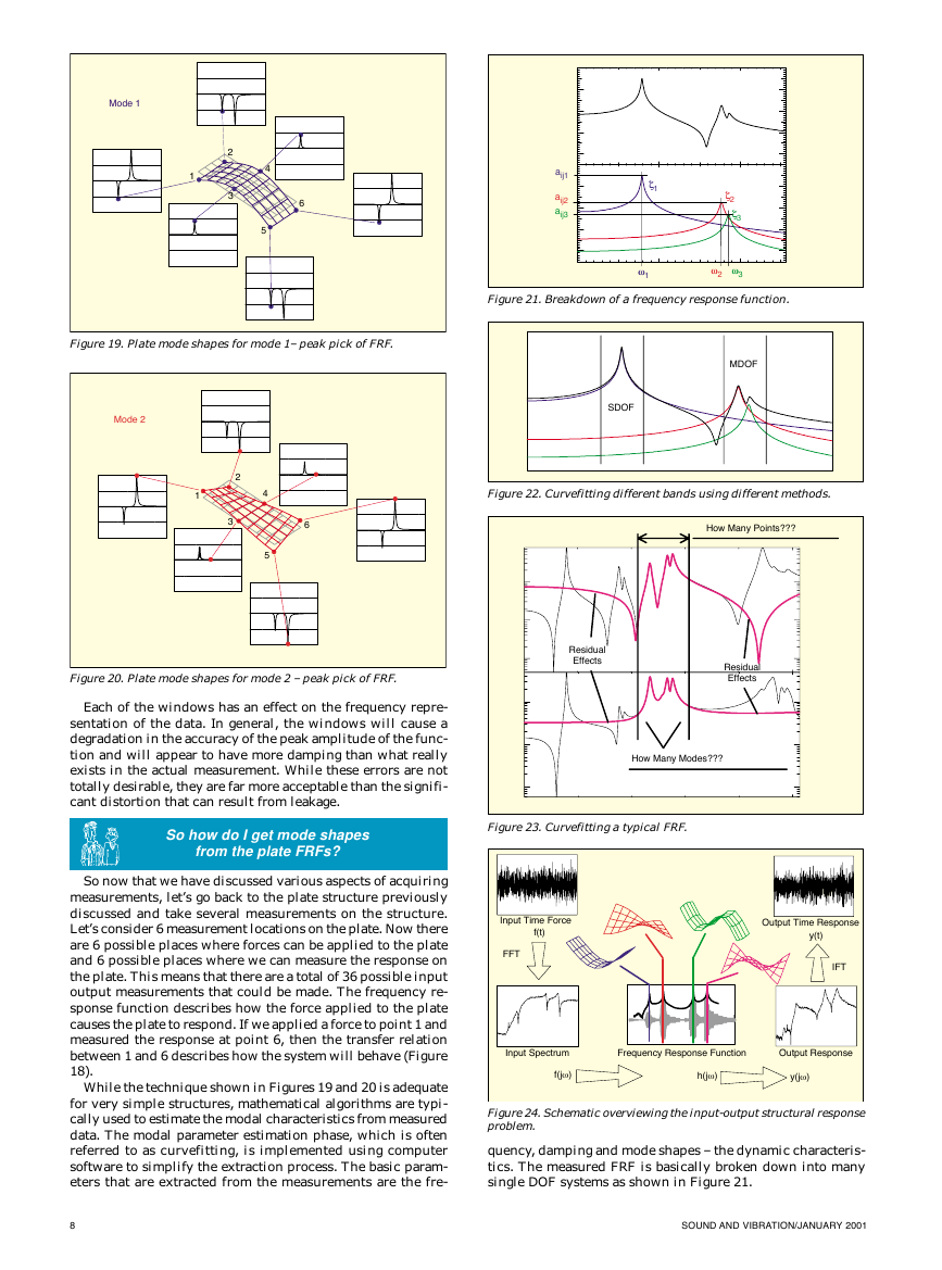
Figure 21. Breakdown of a frequency response function.
MDOF
SDOF
Figure 22. Curvefitting different bands using different methods.
How Many Points???
Figure 20. Plate mode shapes for mode 2 – peak pick of FRF.
Each of the windows has an effect on the frequency repre-
sentation of the data. In general, the windows will cause a
degradation in the accuracy of the peak amplitude of the func-
tion and will appear to have more damping than what really
exists in the actual measurement. While these errors are not
totally desirable, they are far more acceptable than the signifi-
cant distortion that can result from leakage.
Residual
Effects
Residual
Effects
How Many Modes???
So how do I get mode shapes
from the plate FRFs?
Figure 23. Curvefitting a typical FRF.
So now that we have discussed various aspects of acquiring
measurements, let’s go back to the plate structure previously
discussed and take several measurements on the structure.
Let’s consider 6 measurement locations on the plate. Now there
are 6 possible places where forces can be applied to the plate
and 6 possible places where we can measure the response on
the plate. This means that there are a total of 36 possible input
output measurements that could be made. The frequency re-
sponse function describes how the force applied to the plate
causes the plate to respond. If we applied a force to point 1 and
measured the response at point 6, then the transfer relation
between 1 and 6 describes how the system will behave (Figure
18).
While the technique shown in Figures 19 and 20 is adequate
for very simple structures, mathematical algorithms are typi-
cally used to estimate the modal characteristics from measured
data. The modal parameter estimation phase, which is often
referred to as curvefitting, is implemented using computer
software to simplify the extraction process. The basic param-
eters that are extracted from the measurements are the fre-
Input Time Force
f(t)
FFT
Output Time Response
y(t)
IFT
Input Spectrum
Frequency Response Function
Output Response
f(jω)
h(jω)
y(jω)
Figure 24. Schematic overviewing the input-output structural response
problem.
quency, damping and mode shapes – the dynamic characteris-
tics. The measured FRF is basically broken down into many
single DOF systems as shown in Figure 21.
8
SOUND AND VIBRATION/JANUARY 2001
�


 2023年江西萍乡中考道德与法治真题及答案.doc
 2012年重庆南川中考生物真题及答案.doc
 2013年江西师范大学地理学综合及文艺理论基础考研真题.doc
 2020年四川甘孜小升初语文真题及答案I卷.doc
 2020年注册岩土工程师专业基础考试真题及答案.doc
 2023-2024学年福建省厦门市九年级上学期数学月考试题及答案.doc
 2021-2022学年辽宁省沈阳市大东区九年级上学期语文期末试题及答案.doc
 2022-2023学年北京东城区初三第一学期物理期末试卷及答案.doc
 2018上半年江西教师资格初中地理学科知识与教学能力真题及答案.doc
 2012年河北国家公务员申论考试真题及答案-省级.doc
 2020-2021学年江苏省扬州市江都区邵樊片九年级上学期数学第一次质量检测试题及答案.doc
 2022下半年黑龙江教师资格证中学综合素质真题及答案.doc