g2o: A general Framework for (Hyper) Graph Optimization
Giorgio Grisetti, Rainer K¨ummerle, Hauke Strasdat, Kurt Konolige
email: {grisetti,kuemmerl}@informatik.uni-freiburg.de
strasdat@gmail.com konolige@willowgarage.com
March 11, 2017
In this document we describe a C++ framework for performing the optimization of nonlinear least
squares problems that can be embedded as a graph or in a hyper-graph. A hyper-graph is an extension
of a graph where an edge can connect multiple nodes and not only two. Several problems in robotics and
in computer vision require to find the optimum of an error function with respect of a set of parameters.
Examples include, popular applications like SLAM and Bundle adjustment.
In the literature, many approaches have been proposed to address this class of problems. The naive
implementation of standard methods, like Levenberg-Marquardt or Gauss-Newton can lead to acceptable
results for most applications, when the correct parameterization is chosen. However, to achieve the
maximum performances substantial efforts might be required.
g2o stands for General (Hyper) Graph Optimization. The purposes of this framework are the follow-
ing:
• To provide an easy-to-extend and easy-to-use general library for graph optimization that can be
easily applied to different problems,
• To provide people who want to understand SLAM or BA with an easy-to-read implementation that
focuses on the relevant details of the problem specification.
• Achieve state-of-the-art performances, while being as general as possible.
In the remainder of this document we will first characterize the (hyper) graph-embeddable problems,
and we will give an introduction to their solution via the popular Levenberg-Marquardt or Gauss-Newton
algorithms implemented in this library. Subsequently, we will describe the high-level behavior of the
library, and the basic structures. Finally, we will introduce how to implement 2D SLAM as a simple
example.
This document is not a replacement for the in-line documentation. Instead, it is a digest
to help the user/reader to read/browse and extend the code.
Please cite this when using g2o:
R. K¨ummerle, G. Grisetti, H. Strasdat, K. Konolige, and W. Burgard. g2o: A General Framework for
Graph Optimization. In Proc. of the IEEE Int. Conf. on Robotics and Automation (ICRA). Shanghai,
China, May 2011.
1
(Hyper)Graph-Embeddable Optimization Problems
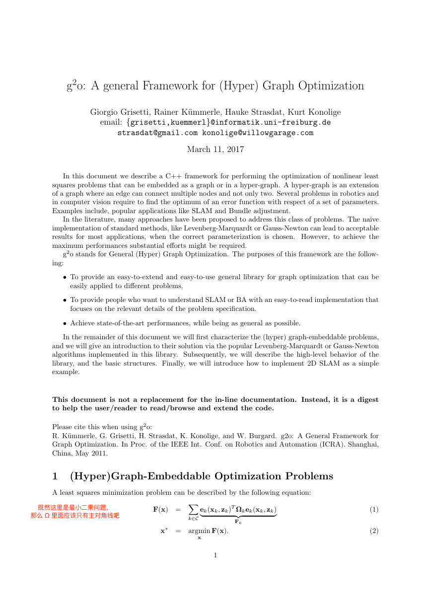
A least squares minimization problem can be described by the following equation:
ek(xk, zk)T Ωkek(xk, zk)
F(x) = Xk∈C
x∗ = argmin
|
x
}
Fk
{z
F(x).
1
(1)
(2)
�
pj
ui−1
pi−1
zij
pi
K
z2i
p0
u0
p1
u1
p2
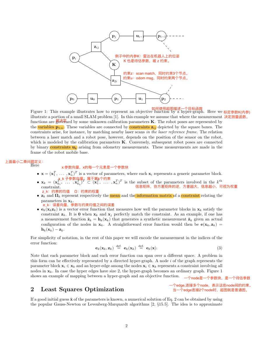
Figure 1: This example illustrates how to represent an objective function by a hyper-graph. Here we
illustrate a portion of a small SLAM problem [1]. In this example we assume that where the measurement
functions are governed by some unknown calibration parameters K. The robot poses are represented by
the variables p1:n. These variables are connected by constraints zij depicted by the square boxes. The
constraints arise, for instance, by matching nearby laser scans in the laser reference frame. The relation
between a laser match and a robot pose, however, depends on the position of the sensor on the robot,
which is modeled by the calibration parameters K. Conversely, subsequent robot poses are connected
by binary constraints uk arising from odometry measurements. These measurements are made in the
frame of the robot mobile base.
Here
• x = (xT
1 , . . . , xT
n )T is a vector of parameters, where each xi represents a generic parameter block.
• xk = (xT
k1
constraint.
,
. . .
, xT
kq
)T ⊂ (xT
1 ,
. . .
, xT
n )T is the subset of the parameters involved in the kth
• zk and Ωk represent respectively the mean and the information matrix of a constraint relating the
parameters in xk.
• ek(xkzk) is a vector error function that measures how well the parameter blocks in xk satisfy the
constraint zk. It is 0 when xk and xj perfectly match the constraint. As an example, if one has
a measurement function ˆzk = hk(xk) that generates a synthetic measurement ˆzk given an actual
configuration of the nodes in xk. A straightforward error function would then be e(xk, zk) =
hk(xk) − zk.
For simplicity of notation, in the rest of this paper we will encode the measurement in the indices of the
error function:
ek(xk, zk) def.= ek(xk) def.= ek(x).
(3)
Note that each parameter block and each error function can span over a different space. A problem in
this form can be effectively represented by a directed hyper-graph. A node i of the graph represents the
parameter block xi ∈ xk and an hyper-edge among the nodes xi ∈ xk represents a constraint involving all
nodes in xk. In case the hyper edges have size 2, the hyper-graph becomes an ordinary graph. Figure 1
shows an example of mapping between a hyper-graph and an objective function.
2 Least Squares Optimization
If a good initial guess ˘x of the parameters is known, a numerical solution of Eq. 2 can be obtained by using
the popular Gauss-Newton or Levenberg-Marquardt algorithms [2, §15.5]. The idea is to approximate
2
�
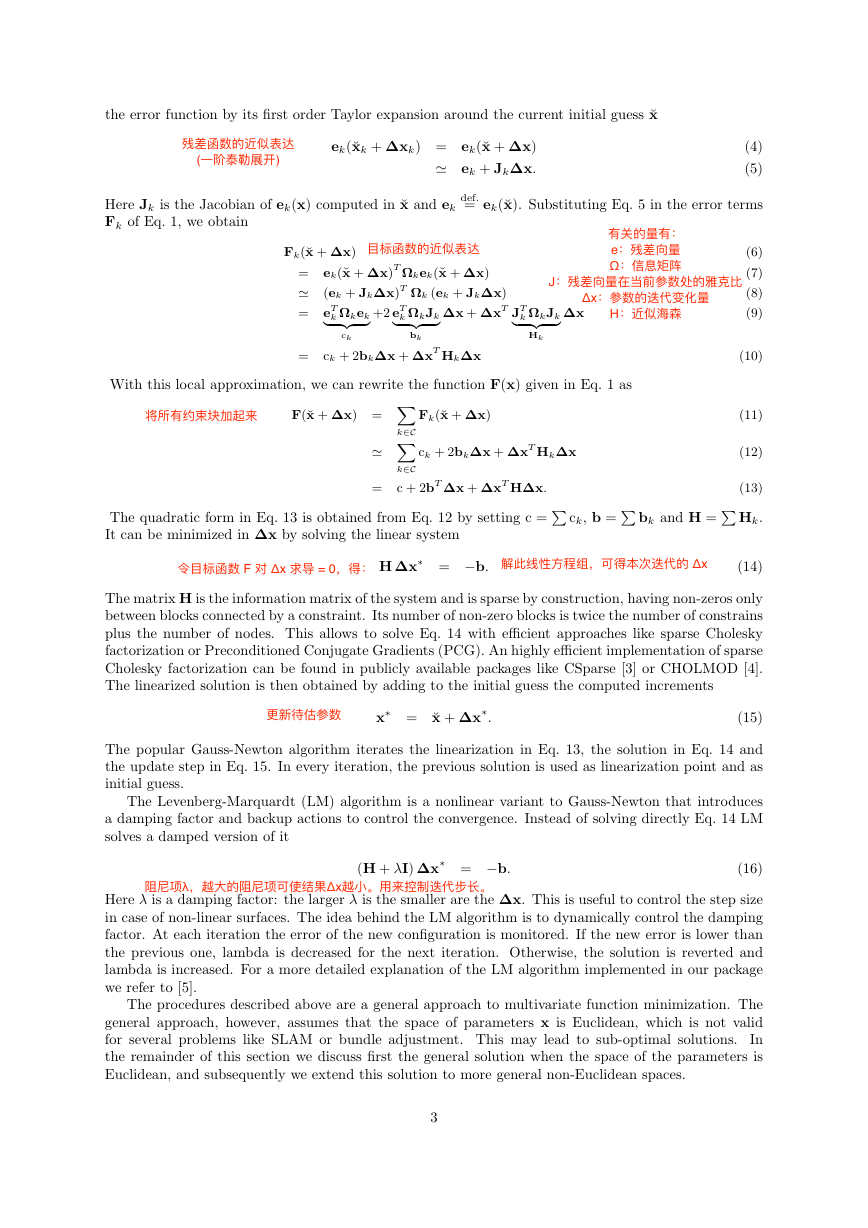
the error function by its first order Taylor expansion around the current initial guess ˘x
ek(˘xk + ∆xk) = ek(˘x + ∆x)
≃ ek + Jk∆x.
(4)
(5)
Here Jk is the Jacobian of ek(x) computed in ˘x and ek
Fk of Eq. 1, we obtain
def.= ek(˘x). Substituting Eq. 5 in the error terms
Fk(˘x + ∆x)
= ek(˘x + ∆x)T Ωkek(˘x + ∆x)
≃ (ek + Jk∆x)T Ωk (ek + Jk∆x)
= eT
|
∆x + ∆xT JT
|
k Ωkek
{z
}
ck
+2 eT
|
k ΩkJk
{z
}
bk
∆x
k ΩkJk
{z
}Hk
With this local approximation, we can rewrite the function F(x) given in Eq. 1 as
= ck + 2bk∆x + ∆xT Hk∆x
F(˘x + ∆x) = X
Fk(˘x + ∆x)
k∈C
≃ X
k∈C
ck + 2bk∆x + ∆xT Hk∆x
= c + 2bT ∆x + ∆xT H∆x.
(6)
(7)
(8)
(9)
(10)
(11)
(12)
(13)
The quadratic form in Eq. 13 is obtained from Eq. 12 by setting c =P ck, b =P bk and H =P Hk.
It can be minimized in ∆x by solving the linear system
H ∆x∗ = −b.
(14)
The matrix H is the information matrix of the system and is sparse by construction, having non-zeros only
between blocks connected by a constraint. Its number of non-zero blocks is twice the number of constrains
plus the number of nodes. This allows to solve Eq. 14 with efficient approaches like sparse Cholesky
factorization or Preconditioned Conjugate Gradients (PCG). An highly efficient implementation of sparse
Cholesky factorization can be found in publicly available packages like CSparse [3] or CHOLMOD [4].
The linearized solution is then obtained by adding to the initial guess the computed increments
x∗ = ˘x + ∆x∗.
(15)
The popular Gauss-Newton algorithm iterates the linearization in Eq. 13, the solution in Eq. 14 and
the update step in Eq. 15. In every iteration, the previous solution is used as linearization point and as
initial guess.
The Levenberg-Marquardt (LM) algorithm is a nonlinear variant to Gauss-Newton that introduces
a damping factor and backup actions to control the convergence. Instead of solving directly Eq. 14 LM
solves a damped version of it
(H + λI) ∆x∗ = −b.
(16)
Here λ is a damping factor: the larger λ is the smaller are the ∆x. This is useful to control the step size
in case of non-linear surfaces. The idea behind the LM algorithm is to dynamically control the damping
factor. At each iteration the error of the new configuration is monitored. If the new error is lower than
the previous one, lambda is decreased for the next iteration. Otherwise, the solution is reverted and
lambda is increased. For a more detailed explanation of the LM algorithm implemented in our package
we refer to [5].
The procedures described above are a general approach to multivariate function minimization. The
general approach, however, assumes that the space of parameters x is Euclidean, which is not valid
for several problems like SLAM or bundle adjustment. This may lead to sub-optimal solutions.
In
the remainder of this section we discuss first the general solution when the space of the parameters is
Euclidean, and subsequently we extend this solution to more general non-Euclidean spaces.
3
�
3 Considerations about the Structure of the Linearized System
According to Eq. 13, the matrix H and the vector b are obtained by summing up a set of matrices and
vectors, one for every constraint. If we set bk = JT
k ΩkJk we can rewrite H and b as
k Ωkek and Hk = JT
b = Xk∈C
H = Xk∈C
bij
Hij.
(17)
(18)
Every constraint will contribute to the system with an addend term. The structure of this addend
depends on the Jacobian of the error function. Since the error function of a constraint depends only on
the values of the nodes xi ∈ xk, the Jacobian in Eq. 5 has the following form:
Jk = 0 · · · 0 Jk1 · · · Jki · · · 0 · · · Jkq 0 · · · 0 .
(19)
Here Jki = ∂e(xk)
∂xki
kth hyper-edge, with respect to the parameter block xki ∈ xk.
are the derivatives of the error function with respect to the nodes connected by the
From Eq. 9 we obtain the following structure for the block matrix Hij:
Hk =
bk =
. . .
JT
k1ΩkJk1
· · ·
JT
k1ΩkJki
· · · JT
k1ΩkJkq
...
ΩkJk1
...
ΩkJk1
JT
ki
JT
kq
...
ΩkBki
...
ΩkBki
· · ·
JT
ki
· · · JT
kq
...
ΩkJkq
...
ΩkJkq
· · ·
JT
ki
· · · JT
kq
...
Jk1Ωkek
JT
ki
JT
kq
...
Ωkek
...
Ωkek
...
. . .
(20)
(21)
For simplicity of notation we omitted the zero blocks. The reader might notice that the block structure
of the matrix H is the adjacency matrix of the hyper graph. Additionally the Hessian H is a symmetric
matrix, since all the Hk are symmetric. A single hyper-edge connecting q vertices will introduce q2 non
zero blocks in the Hessian, in correspondence of each pair xki , xkj, of nodes connected.
4 Least Squares on Manifold
To deal with parameter blocks that span over a non-Euclidean spaces, it is common to apply the error
minimization on a manifold. A manifold is a mathematical space that is not necessarily Euclidean on a
global scale, but can be seen as Euclidean on a local scale [6].
For example, in the context of SLAM problem, each parameter block xi consists of a translation vector
ti and a rotational component αi. The translation ti clearly forms a Euclidean space. In contrast to that,
the rotational components αi span over the non-Euclidean 2D or 3D rotation group SO(2) or SO(3).
To avoid singularities, these spaces are usually described in an over-parameterized way, e.g., by rotation
matrices or quaternions. Directly applying Eq. 15 to these over-parameterized representations breaks
the constraints induced by the over-parameterization. The over-parameterization results in additional
4
�
degrees of freedom and thus introduces errors in the solution. To overcome this problem, one can use
a minimal representation for the rotation (like Euler angles in 3D). This, however, is then subject to
singularities.
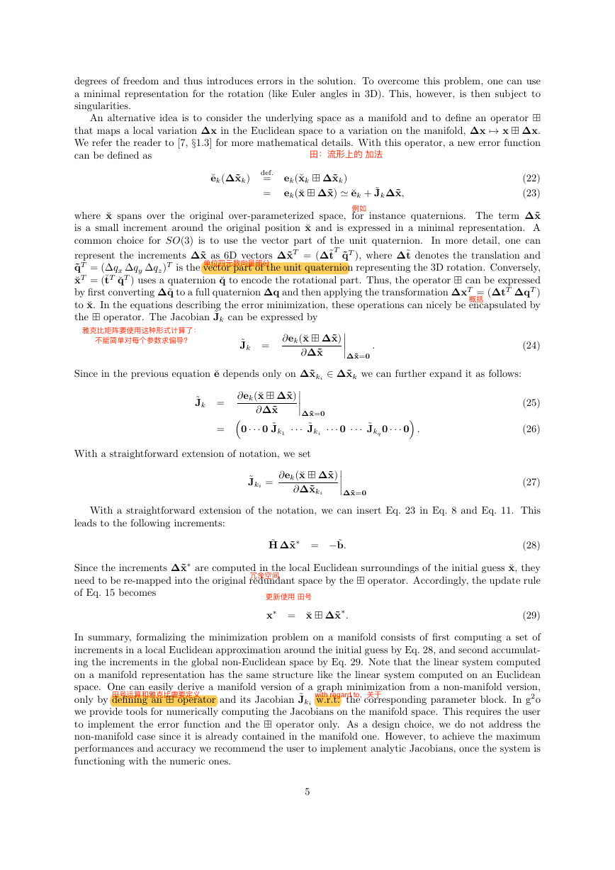
An alternative idea is to consider the underlying space as a manifold and to define an operator ⊞
that maps a local variation ∆x in the Euclidean space to a variation on the manifold, ∆x 7→ x ⊞ ∆x.
We refer the reader to [7, §1.3] for more mathematical details. With this operator, a new error function
can be defined as
˘ek(∆˜xk)
def.= ek(˘xk ⊞ ∆˜xk)
= ek(˘x ⊞ ∆˜x) ≃ ˘ek + ˜Jk∆˜x,
(22)
(23)
where ˘x spans over the original over-parameterized space, for instance quaternions. The term ∆˜x
is a small increment around the original position ˘x and is expressed in a minimal representation. A
common choice for SO(3) is to use the vector part of the unit quaternion.
In more detail, one can
T
represent the increments ∆˜x as 6D vectors ∆˜xT = (∆˜t
˜qT ), where ∆˜t denotes the translation and
˜qT = (∆qx ∆qy ∆qz)T is the vector part of the unit quaternion representing the 3D rotation. Conversely,
˘xT = (˘tT ˘qT ) uses a quaternion ˘q to encode the rotational part. Thus, the operator ⊞ can be expressed
by first converting ∆˜q to a full quaternion ∆q and then applying the transformation ∆xT = (∆tT ∆qT )
to ˘x. In the equations describing the error minimization, these operations can nicely be encapsulated by
the ⊞ operator. The Jacobian ˜Jk can be expressed by
Since in the previous equation ˘e depends only on ∆˜xki ∈ ∆˜xk we can further expand it as follows:
˜Jk =
∂ek(˘x ⊞ ∆˜x)
∂∆˜x
.
∆˜x=0
˜Jk =
∂ek(˘x ⊞ ∆˜x)
∂∆˜x
∆˜x=0
= 0 · · · 0 ˜Jk1 · · · ˜Jki · · · 0 · · · ˜Jkq 0 · · · 0 .
With a straightforward extension of notation, we set
(24)
(25)
(26)
(27)
˜Jki =
∂ek(˘x ⊞ ∆˜x)
∂∆˜xki
∆˜x=0
With a straightforward extension of the notation, we can insert Eq. 23 in Eq. 8 and Eq. 11. This
leads to the following increments:
˜H ∆˜x∗ = −˜b.
(28)
Since the increments ∆˜x∗ are computed in the local Euclidean surroundings of the initial guess ˘x, they
need to be re-mapped into the original redundant space by the ⊞ operator. Accordingly, the update rule
of Eq. 15 becomes
x∗ = ˘x ⊞ ∆˜x∗.
(29)
In summary, formalizing the minimization problem on a manifold consists of first computing a set of
increments in a local Euclidean approximation around the initial guess by Eq. 28, and second accumulat-
ing the increments in the global non-Euclidean space by Eq. 29. Note that the linear system computed
on a manifold representation has the same structure like the linear system computed on an Euclidean
space. One can easily derive a manifold version of a graph minimization from a non-manifold version,
only by defining an ⊞ operator and its Jacobian ˜Jki w.r.t. the corresponding parameter block. In g2o
we provide tools for numerically computing the Jacobians on the manifold space. This requires the user
to implement the error function and the ⊞ operator only. As a design choice, we do not address the
non-manifold case since it is already contained in the manifold one. However, to achieve the maximum
performances and accuracy we recommend the user to implement analytic Jacobians, once the system is
functioning with the numeric ones.
5
�
5 Robust Least Squares
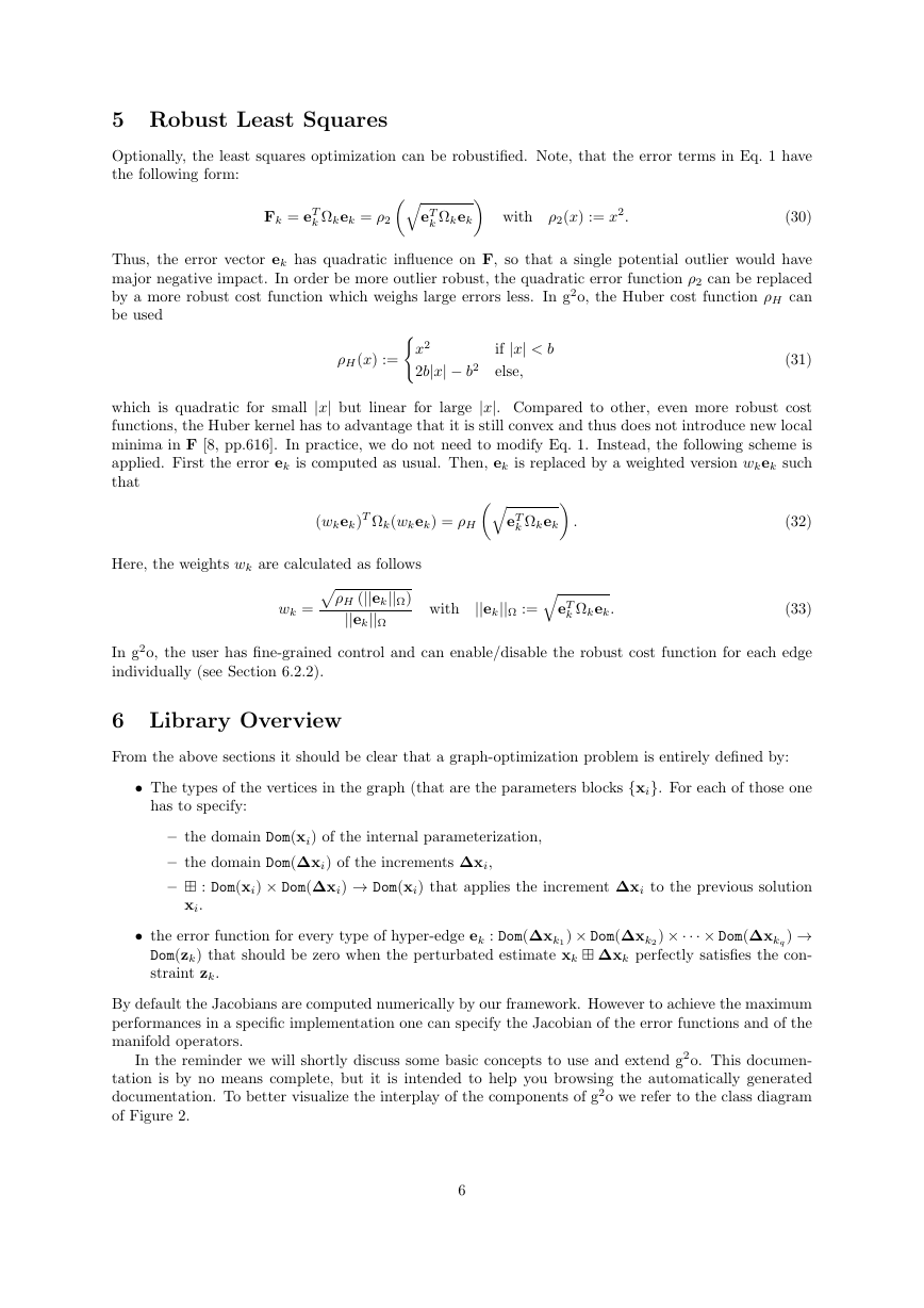
Optionally, the least squares optimization can be robustified. Note, that the error terms in Eq. 1 have
the following form:
Fk = eT
k Ωkek = ρ2qeT
k Ωkek with ρ2(x) := x2.
(30)
Thus, the error vector ek has quadratic influence on F, so that a single potential outlier would have
major negative impact. In order be more outlier robust, the quadratic error function ρ2 can be replaced
by a more robust cost function which weighs large errors less. In g2o, the Huber cost function ρH can
be used
ρH (x) :=(x2
2b|x| − b2
if |x| < b
else,
(31)
which is quadratic for small |x| but linear for large |x|. Compared to other, even more robust cost
functions, the Huber kernel has to advantage that it is still convex and thus does not introduce new local
minima in F [8, pp.616]. In practice, we do not need to modify Eq. 1. Instead, the following scheme is
applied. First the error ek is computed as usual. Then, ek is replaced by a weighted version wkek such
that
(wkek)T Ωk(wkek) = ρHqeT
k Ωkek .
Here, the weights wk are calculated as follows
wk = pρH (||ek||Ω)
||ek||Ω
with ||ek||Ω :=qeT
k Ωkek.
(32)
(33)
In g2o, the user has fine-grained control and can enable/disable the robust cost function for each edge
individually (see Section 6.2.2).
6 Library Overview
From the above sections it should be clear that a graph-optimization problem is entirely defined by:
• The types of the vertices in the graph (that are the parameters blocks {xi}. For each of those one
has to specify:
– the domain Dom(xi) of the internal parameterization,
– the domain Dom(∆xi) of the increments ∆xi,
– ⊞ : Dom(xi) × Dom(∆xi) → Dom(xi) that applies the increment ∆xi to the previous solution
xi.
• the error function for every type of hyper-edge ek : Dom(∆xk1) × Dom(∆xk2) × · · · × Dom(∆xkq ) →
Dom(zk) that should be zero when the perturbated estimate xk ⊞ ∆xk perfectly satisfies the con-
straint zk.
By default the Jacobians are computed numerically by our framework. However to achieve the maximum
performances in a specific implementation one can specify the Jacobian of the error functions and of the
manifold operators.
In the reminder we will shortly discuss some basic concepts to use and extend g2o. This documen-
tation is by no means complete, but it is intended to help you browsing the automatically generated
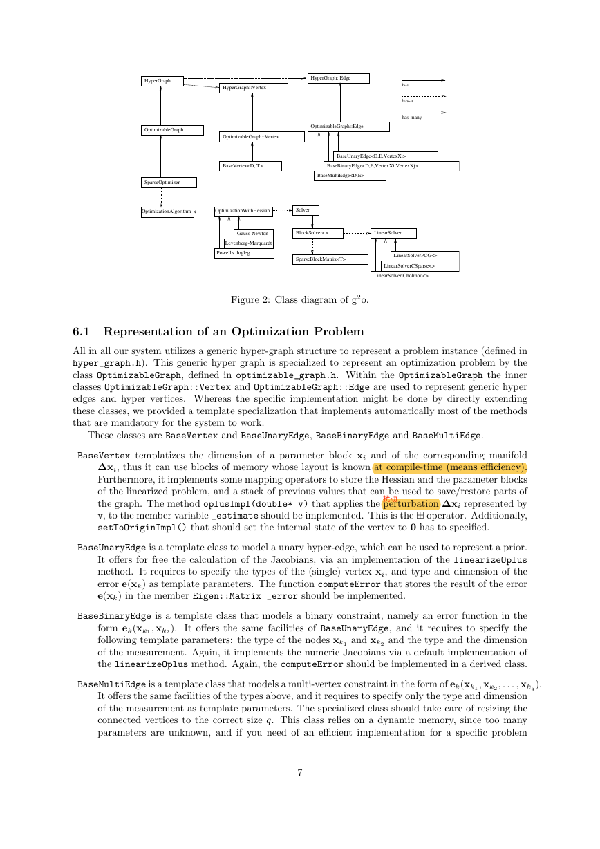
documentation. To better visualize the interplay of the components of g2o we refer to the class diagram
of Figure 2.
6
�
HyperGraph
HyperGraph::Vertex
HyperGraph::Edge
is-a
has-a
has-many
OptimizableGraph
OptimizableGraph::Vertex
OptimizableGraph::Edge
BaseVertex
BaseBinaryEdge
BaseUnaryEdge
BaseMultiEdge
SparseOptimizer
OptimizationAlgorithm
OptimizationWithHessian
Solver
Gauss-Newton
BlockSolver<>
LinearSolver
Levenberg-Marquardt
Powell's dogleg
SparseBlockMatrix
LinearSolverPCG<>
LinearSolverCSparse<>
LinearSolverlCholmod<>
Figure 2: Class diagram of g2o.
6.1 Representation of an Optimization Problem
All in all our system utilizes a generic hyper-graph structure to represent a problem instance (defined in
hyper_graph.h). This generic hyper graph is specialized to represent an optimization problem by the
class OptimizableGraph, defined in optimizable_graph.h. Within the OptimizableGraph the inner
classes OptimizableGraph::Vertex and OptimizableGraph::Edge are used to represent generic hyper
edges and hyper vertices. Whereas the specific implementation might be done by directly extending
these classes, we provided a template specialization that implements automatically most of the methods
that are mandatory for the system to work.
These classes are BaseVertex and BaseUnaryEdge, BaseBinaryEdge and BaseMultiEdge.
BaseVertex templatizes the dimension of a parameter block xi and of the corresponding manifold
∆xi, thus it can use blocks of memory whose layout is known at compile-time (means efficiency).
Furthermore, it implements some mapping operators to store the Hessian and the parameter blocks
of the linearized problem, and a stack of previous values that can be used to save/restore parts of
the graph. The method oplusImpl(double* v) that applies the perturbation ∆xi represented by
v, to the member variable _estimate should be implemented. This is the ⊞ operator. Additionally,
setToOriginImpl() that should set the internal state of the vertex to 0 has to specified.
BaseUnaryEdge is a template class to model a unary hyper-edge, which can be used to represent a prior.
It offers for free the calculation of the Jacobians, via an implementation of the linearizeOplus
method. It requires to specify the types of the (single) vertex xi, and type and dimension of the
error e(xk) as template parameters. The function computeError that stores the result of the error
e(xk) in the member Eigen::Matrix _error should be implemented.
BaseBinaryEdge is a template class that models a binary constraint, namely an error function in the
form ek(xk1 , xk2 ). It offers the same facilities of BaseUnaryEdge, and it requires to specify the
following template parameters: the type of the nodes xk1 and xk2 and the type and the dimension
of the measurement. Again, it implements the numeric Jacobians via a default implementation of
the linearizeOplus method. Again, the computeError should be implemented in a derived class.
BaseMultiEdge is a template class that models a multi-vertex constraint in the form of ek(xk1 , xk2 , . . . , xkq ).
It offers the same facilities of the types above, and it requires to specify only the type and dimension
of the measurement as template parameters. The specialized class should take care of resizing the
connected vertices to the correct size q. This class relies on a dynamic memory, since too many
parameters are unknown, and if you need of an efficient implementation for a specific problem
7
�
#i n c l u d e ” g2o / c o r e / f a c t o r y . h”
namespace g2o {
G2O REGISTER TYPE GROUP( slam2d ) ;
G2O REGISTER TYPE(VERTEX SE2, VertexSE2 ) ;
G2O REGISTER TYPE(VERTEX XY, VertexPointXY ) ;
// . . .
}
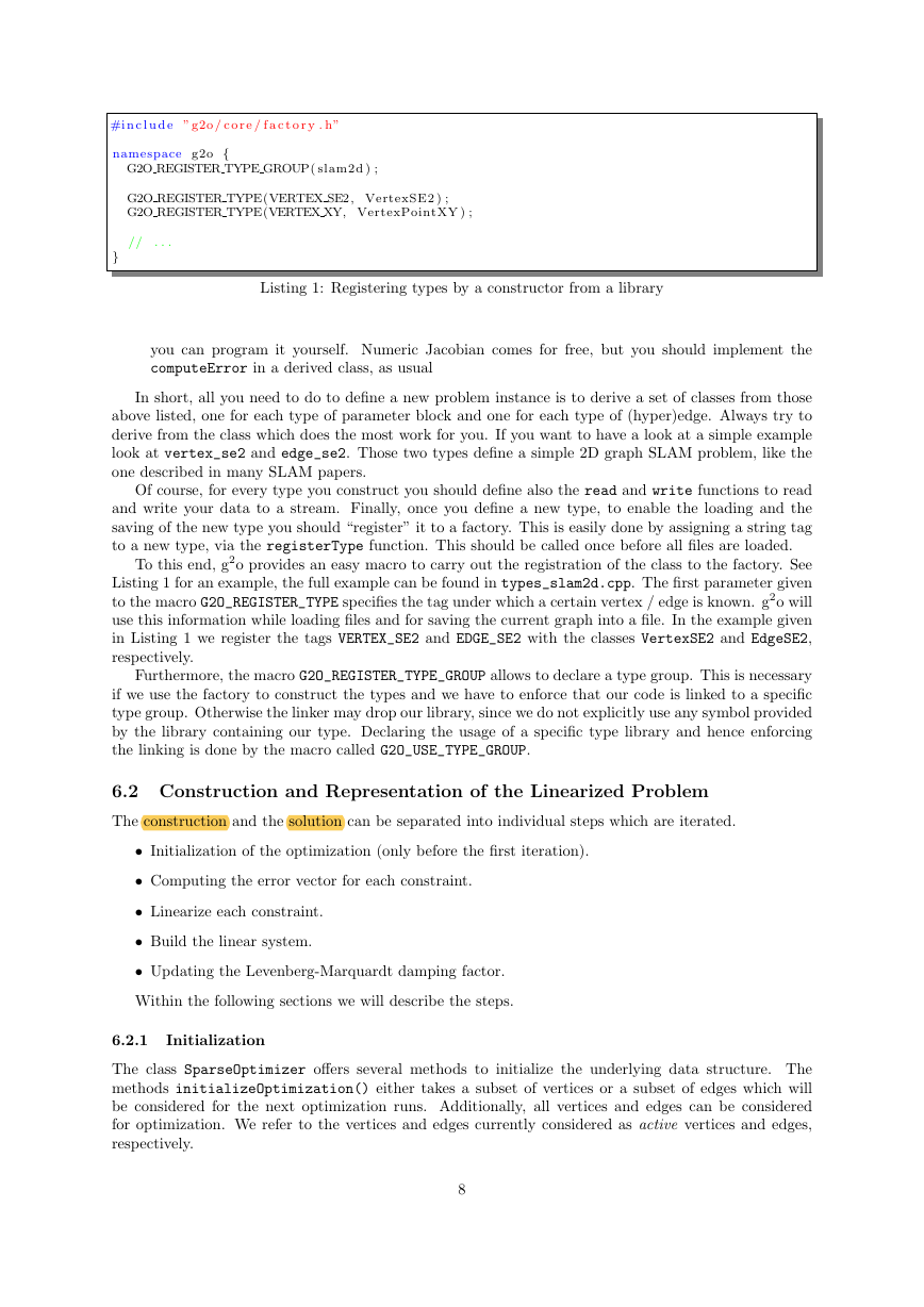
Listing 1: Registering types by a constructor from a library
you can program it yourself. Numeric Jacobian comes for free, but you should implement the
computeError in a derived class, as usual
In short, all you need to do to define a new problem instance is to derive a set of classes from those
above listed, one for each type of parameter block and one for each type of (hyper)edge. Always try to
derive from the class which does the most work for you. If you want to have a look at a simple example
look at vertex_se2 and edge_se2. Those two types define a simple 2D graph SLAM problem, like the
one described in many SLAM papers.
Of course, for every type you construct you should define also the read and write functions to read
and write your data to a stream. Finally, once you define a new type, to enable the loading and the
saving of the new type you should “register” it to a factory. This is easily done by assigning a string tag
to a new type, via the registerType function. This should be called once before all files are loaded.
To this end, g2o provides an easy macro to carry out the registration of the class to the factory. See
Listing 1 for an example, the full example can be found in types_slam2d.cpp. The first parameter given
to the macro G2O_REGISTER_TYPE specifies the tag under which a certain vertex / edge is known. g2o will
use this information while loading files and for saving the current graph into a file. In the example given
in Listing 1 we register the tags VERTEX_SE2 and EDGE_SE2 with the classes VertexSE2 and EdgeSE2,
respectively.
Furthermore, the macro G2O_REGISTER_TYPE_GROUP allows to declare a type group. This is necessary
if we use the factory to construct the types and we have to enforce that our code is linked to a specific
type group. Otherwise the linker may drop our library, since we do not explicitly use any symbol provided
by the library containing our type. Declaring the usage of a specific type library and hence enforcing
the linking is done by the macro called G2O_USE_TYPE_GROUP.
6.2 Construction and Representation of the Linearized Problem
The construction and the solution can be separated into individual steps which are iterated.
• Initialization of the optimization (only before the first iteration).
• Computing the error vector for each constraint.
• Linearize each constraint.
• Build the linear system.
• Updating the Levenberg-Marquardt damping factor.
Within the following sections we will describe the steps.
6.2.1
Initialization
The class SparseOptimizer offers several methods to initialize the underlying data structure. The
methods initializeOptimization() either takes a subset of vertices or a subset of edges which will
be considered for the next optimization runs. Additionally, all vertices and edges can be considered
for optimization. We refer to the vertices and edges currently considered as active vertices and edges,
respectively.
8
�



 2023年江西萍乡中考道德与法治真题及答案.doc
 2012年重庆南川中考生物真题及答案.doc
 2013年江西师范大学地理学综合及文艺理论基础考研真题.doc
 2020年四川甘孜小升初语文真题及答案I卷.doc
 2020年注册岩土工程师专业基础考试真题及答案.doc
 2023-2024学年福建省厦门市九年级上学期数学月考试题及答案.doc
 2021-2022学年辽宁省沈阳市大东区九年级上学期语文期末试题及答案.doc
 2022-2023学年北京东城区初三第一学期物理期末试卷及答案.doc
 2018上半年江西教师资格初中地理学科知识与教学能力真题及答案.doc
 2012年河北国家公务员申论考试真题及答案-省级.doc
 2020-2021学年江苏省扬州市江都区邵樊片九年级上学期数学第一次质量检测试题及答案.doc
 2022下半年黑龙江教师资格证中学综合素质真题及答案.doc