1 SURF: Speeded Up Robust Features
In this section, the SURF detector-descriptor scheme is discussed in detail. First the
algorithm is analysed from a theoretical standpoint to provide a detailed overview of how
and why it works. Next the design and development choices for the implementation of
the library are discussed and justified. During the implementation of the library, it was
found that some of the finer details of the algorithm had been omitted or overlooked,
so Section 1.5 serves to make clear the concepts which are not explicitly defined in the
SURF paper [1].
1.1 Integral Images
Much of the performance increase in SURF can be attributed to the use of an intermediate
image representation known as the “Integral Image” [18]. The integral image is computed
rapidly from an input image and is used to speed up the calculation of any upright
rectangular area. Given an input image I and a point (x, y) the integral image I is
calculated by the sum of the values between the point and the origin. Formally this can
be defined by the formula:
i≤x
j≤y
I(x, y) =
I(x, y)
(1)
i=0
j=0
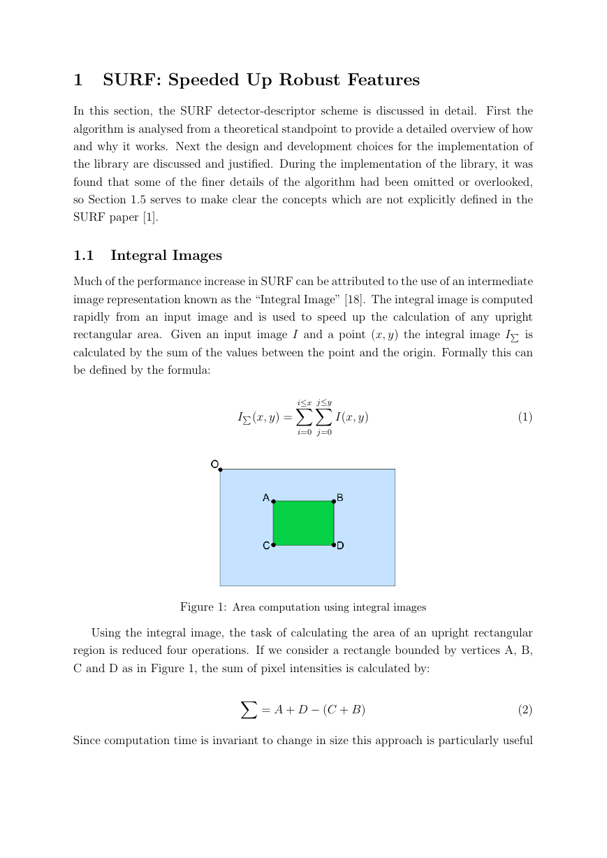
Figure 1: Area computation using integral images
Using the integral image, the task of calculating the area of an upright rectangular
region is reduced four operations. If we consider a rectangle bounded by vertices A, B,
C and D as in Figure 1, the sum of pixel intensities is calculated by:
= A + D − (C + B)
(2)
Since computation time is invariant to change in size this approach is particularly useful
�
when large areas are required. SURF makes good use of this property to perform fast
convolutions of varying size box filters at near constant time.
1.2 Fast-Hessian Detector
1.2.1 The Hessian
The SURF detector is based on the determinant of the Hessian matrix.
In order to
motivate the use of the Hessian, we consider a continuous function of two variables such
that the value of the function at (x, y) is given by f (x, y). The Hessian matrix, H, is the
matrix of partial derivates of the function f .
∂2f
H(f (x, y)) =
∂x2
∂2f
∂x∂y
∂2f
∂x∂y
∂2f
∂y2
∂2f
2
(3)
(4)
The determinant of this matrix, known as the discriminant, is calculated by:
det(H) =
∂2f
∂x2
∂2f
∂y2 −
∂x∂y
The value of the discriminant is used to classify the maxima and minima of the
function by the second order derivative test. Since the determinant is the product of
eigenvalues of the Hessian we can classify the points based on the sign of the result. If
the determinant is negative then the eigenvalues have different signs and hence the point
is not a local extremum; if it is positive then either both eigenvalues are positive or both
are negative and in either case the point is classified as an extremum.
Translating this theory to work with images rather than a continuous function is a
fairly trivial task. First we replace the function values f (x, y) by the image pixel intensi-
ties I(x, y). Next we require a method to calculate the second order partial derivatives of
the image. As described in Section ?? we can calculate derivatives by convolution with
an appropriate kernel. In the case of SURF the second order scale normalised Gaussian is
the chosen filter as it allows for analysis over scales as well as space (scale-space theory is
discussed further later in this section). We can construct kernels for the Gaussian deriva-
tives in x, y and combined xy direction such that we calculate the four entries of the
Hessian matrix. Use of the Gaussian allows us to vary the amount of smoothing during
the convolution stage so that the determinant is calculated at different scales. Further-
more, since the Gaussian is an isotropic (i.e. circularly symmetric) function, convolution
with the kernel allows for rotation invariance. We can now calculate the Hessian matrix,
H, as function of both space x = (x, y) and scale σ.
�
H(x, σ) =
,
Lxx(x, σ) Lxy(x, σ)
Lxy(x, σ) Lyy(x, σ)
(5)
Here Lxx(x, σ) refers to the convolution of the second order Gaussian derivative ∂2g(σ)
∂x2
with the image at point x = (x, y) and similarly for Lyy and Lxy. These derivatives are
known as Laplacian of Gaussians.
Working from this we can calculate the determinant of the Hessian for each pixel in
the image and use the value to find interest points. This variation of the Hessian detector
is similar to that proposed by Beaudet [2].
Lowe [9] found performance increase in approximating the Laplacian of Gaussians by
a difference of Gaussians. In a similiar manner, Bay [1] proposed an approximation to
the Laplacian of Gaussians by using box filter representations of the respective kernels.
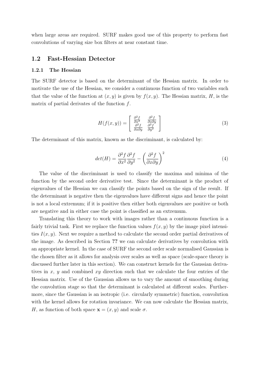
Figure 2 illustrates the similarity between the discretised and cropped kernels and their
box filter counterparts. Considerable performance increase is found when these filters
are used in conjunction with the integral image described in Section 1.1. To qauntify
the difference we can consider the number of array accesses and operations required in
the convolution. For a 9 × 9 filter we would require 81 array accesses and operations for
the original real valued filter and only 8 for the box filter representation. As the filter is
increased in size, the computation cost increases significantly for the original Laplacian
while the cost for the box filters is independent of size.
Figure 2: Laplacian of Gaussian Approximation. Top Row: The discretised and cropped second
order Gaussian derivatives in the x, y and xy-directions. We refer to these as Lxx, Lyy, Lxy.
Bottom Row: Weighted Box filter approximations in the x, y and xy-directions. We refer to
these as Dxx, Dyy, Dxy
In Figure 2 the weights applied to each of the filter sections is kept simple. The
black regions are weighted with a value of 1, the white regions with a value of -1 and the
�
remaining areas not weighted at all. Simple weighting allows for rapid calculation of areas
but in using these weights we need to address the difference in response values between
the original and approximated kernels. Bay [1] proposes the following formula as an
accurate approximation for the Hessian determinant using the approximated Gaussians:
det(Happrox) = DxxDyy − (0.9Dxy)2
(6)
In [1] the two filters are compared in detail and the results conclude that the box
representation’s negligible loss in accuracy is far outweighed by the considerable increase
in efficiency and speed. The determinant here is referred to as the blob response at
location x = (x, y, σ). The search for local maxima of this function over both space and
scale yields the interest points for an image. The exact method for extracting interest
points is explained in the following section.
1.2.2 Constructing the Scale-Space
In order to detect interest points using the determinant of Hessian it is first necessary to
introduce the notion of a scale-space. A scale-space is a continuous function which can be
used to find extrema across all possible scales [20]. In computer vision the scale-space is
typically implemented as an image pyramid where the input image is iteratively convolved
with Gaussian kernel and repeatedly sub-sampled (reduced in size). This method is used
to great effect in SIFT [9] but since each layer relies on the previous, and images need
to be resized it is not computationally efficient. As the processing time of the kernels
used in SURF is size invariant, the scale-space can be created by applying kernels of
increasing size to the original image. This allows for multiple layers of the scale-space
pyramid to be processed simultaneously and negates the need to subsample the image
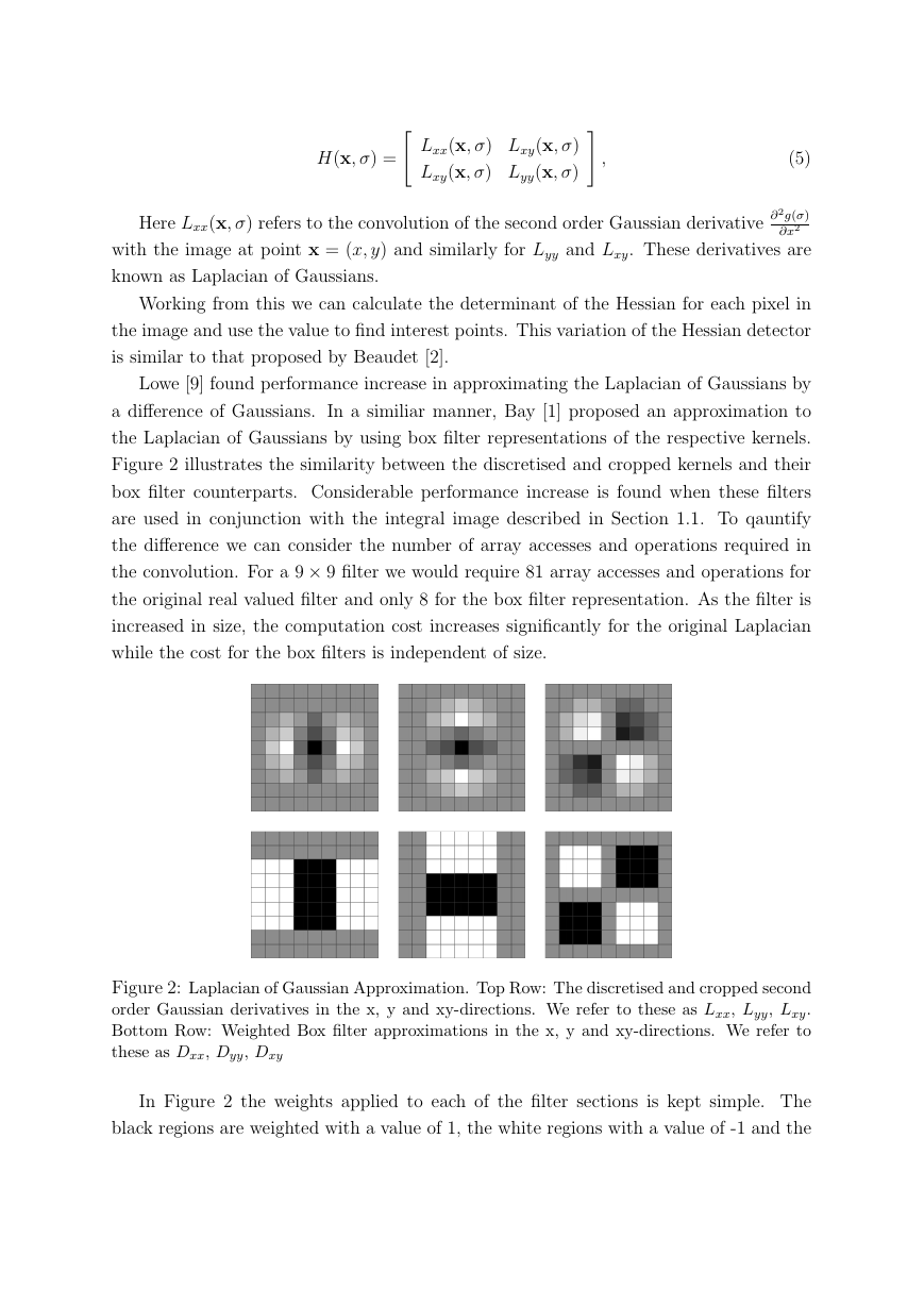
hence providing performance increase. Figure 3 illustrates the difference between the
traditional scale-space structure and the SURF counterpart.
Figure 3: Filter Pyramid. The traditional approach to constructing a scale-space (left).
The image size is varied and the Guassian filter is repeatedly applied to smooth subse-
quent layers. The SURF approach (right) leaves the original image unchanged and varies
only the filter size.
�
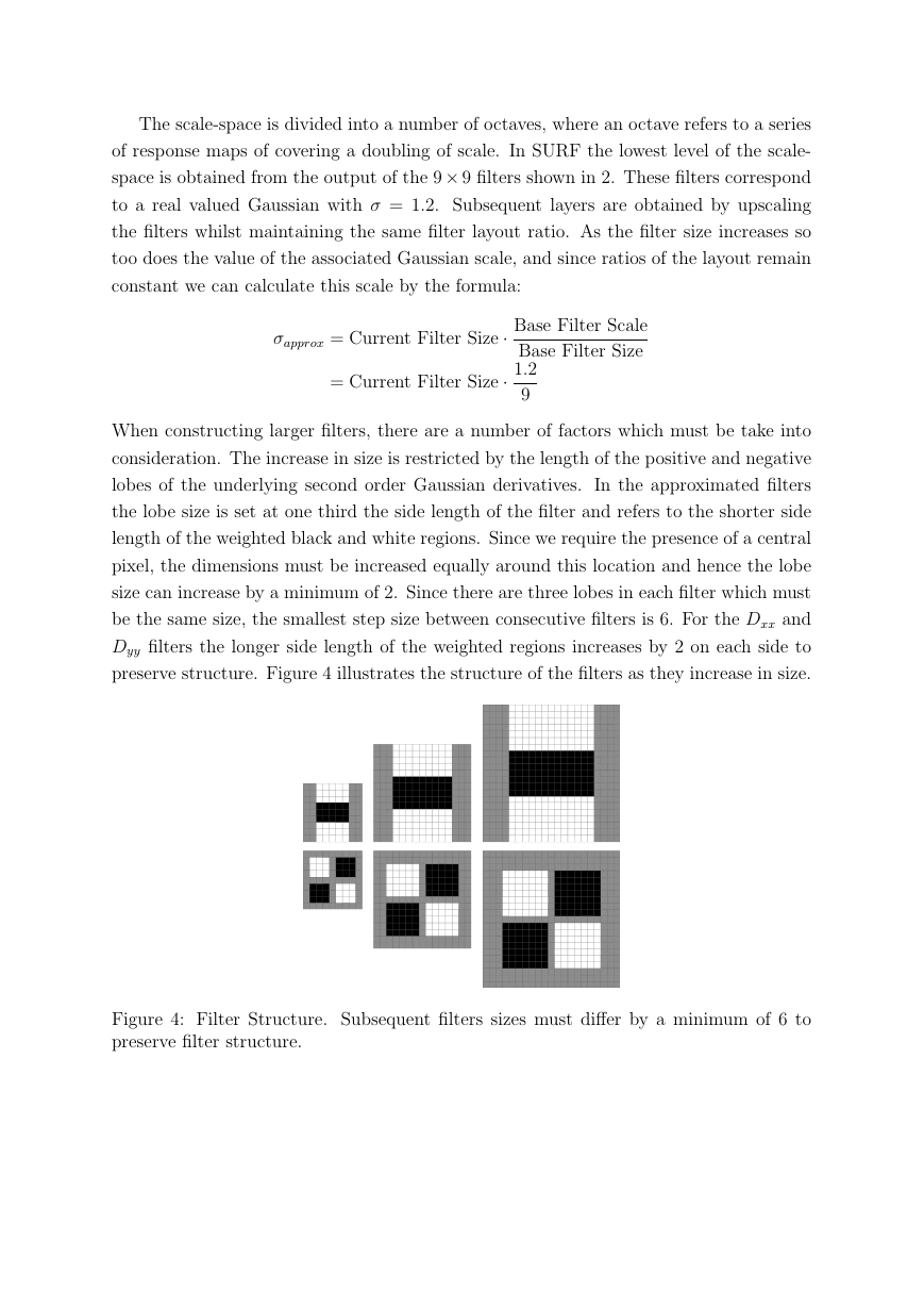
The scale-space is divided into a number of octaves, where an octave refers to a series
of response maps of covering a doubling of scale. In SURF the lowest level of the scale-
space is obtained from the output of the 9× 9 filters shown in 2. These filters correspond
to a real valued Gaussian with σ = 1.2. Subsequent layers are obtained by upscaling
the filters whilst maintaining the same filter layout ratio. As the filter size increases so
too does the value of the associated Gaussian scale, and since ratios of the layout remain
constant we can calculate this scale by the formula:
σapprox = Current Filter Size · Base Filter Scale
Base Filter Size
= Current Filter Size · 1.2
9
When constructing larger filters, there are a number of factors which must be take into
consideration. The increase in size is restricted by the length of the positive and negative
lobes of the underlying second order Gaussian derivatives. In the approximated filters
the lobe size is set at one third the side length of the filter and refers to the shorter side
length of the weighted black and white regions. Since we require the presence of a central
pixel, the dimensions must be increased equally around this location and hence the lobe
size can increase by a minimum of 2. Since there are three lobes in each filter which must
be the same size, the smallest step size between consecutive filters is 6. For the Dxx and
Dyy filters the longer side length of the weighted regions increases by 2 on each side to
preserve structure. Figure 4 illustrates the structure of the filters as they increase in size.
Figure 4: Filter Structure. Subsequent filters sizes must differ by a minimum of 6 to
preserve filter structure.
�
1.2.3 Accurate Interest Point Localisation
The task of localising the scale and rotation invariant interest points in the image can be
divided into three steps. First the responses are thresholded such that all values below
the predetermined threshold are removed. Increasing the threshold lowers the number
of detected interest points, leaving only the strongest while decreasing allows for many
more to detected. Therefore the threshold can be adapted to tailor the detection to the
application.
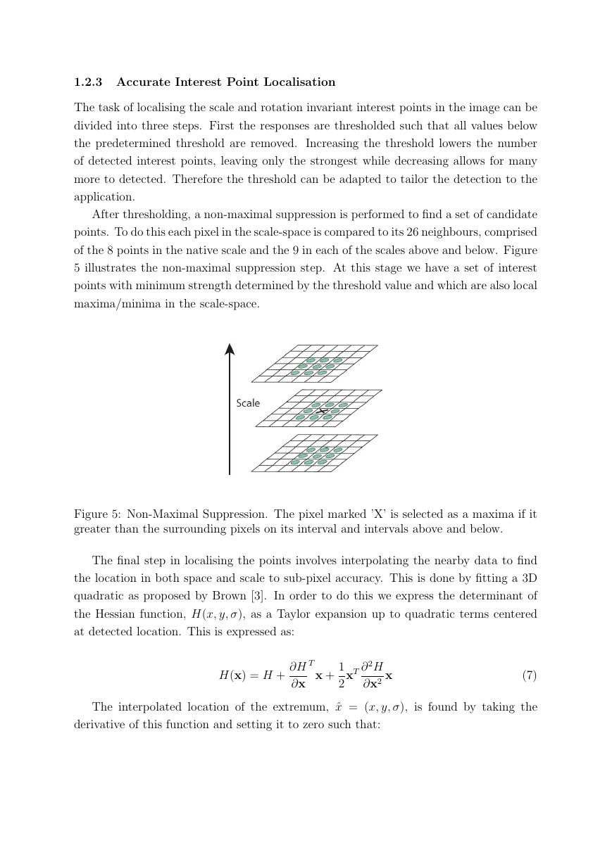
After thresholding, a non-maximal suppression is performed to find a set of candidate
points. To do this each pixel in the scale-space is compared to its 26 neighbours, comprised
of the 8 points in the native scale and the 9 in each of the scales above and below. Figure
5 illustrates the non-maximal suppression step. At this stage we have a set of interest
points with minimum strength determined by the threshold value and which are also local
maxima/minima in the scale-space.
Figure 5: Non-Maximal Suppression. The pixel marked ’X’ is selected as a maxima if it
greater than the surrounding pixels on its interval and intervals above and below.
The final step in localising the points involves interpolating the nearby data to find
the location in both space and scale to sub-pixel accuracy. This is done by fitting a 3D
quadratic as proposed by Brown [3]. In order to do this we express the determinant of
the Hessian function, H(x, y, σ), as a Taylor expansion up to quadratic terms centered
at detected location. This is expressed as:
H(x) = H +
T
∂H
∂x
x +
1
2
xT ∂2H
∂x2 x
(7)
The interpolated location of the extremum, ˆx = (x, y, σ), is found by taking the
derivative of this function and setting it to zero such that:
�
ˆx = −∂2H
∂x2
−1 ∂H
∂x
(8)
The derivatives here are approximated by finite differences of neighbouring pixels. If ˆx
is greater than 0.5 in the x, y or σ directions we adjust the location and perform the
interpolation again. This procedure is repeated until ˆx is less than 0.5 in all directions
or the the number of predetermined interpolation steps has been exceeded. Those points
which do not converge are dropped from the set of interest points leaving only the most
stable and repeatable.
1.3 Interest Point Descriptor
The SURF descriptor describes how the pixel intensities are distributed within a scale
dependent neighbourhood of each interest point detected by the Fast-Hessian. This ap-
proach is similar to that of SIFT [9] but integral images used in conjunction with filters
known as Haar wavelets are used in order to increase robustness and decrease computa-
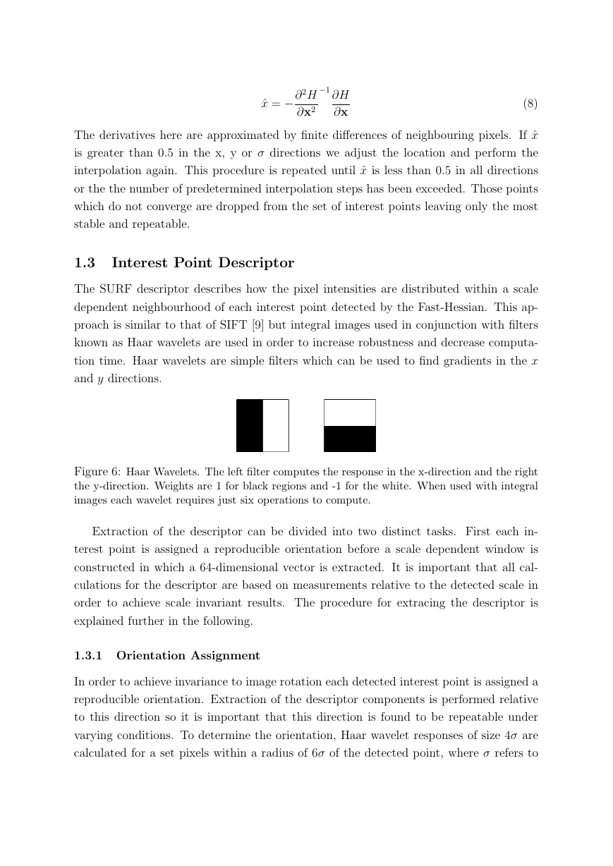
tion time. Haar wavelets are simple filters which can be used to find gradients in the x
and y directions.
Figure 6: Haar Wavelets. The left filter computes the response in the x-direction and the right
the y-direction. Weights are 1 for black regions and -1 for the white. When used with integral
images each wavelet requires just six operations to compute.
Extraction of the descriptor can be divided into two distinct tasks. First each in-
terest point is assigned a reproducible orientation before a scale dependent window is
constructed in which a 64-dimensional vector is extracted. It is important that all cal-
culations for the descriptor are based on measurements relative to the detected scale in
order to achieve scale invariant results. The procedure for extracing the descriptor is
explained further in the following.
1.3.1 Orientation Assignment
In order to achieve invariance to image rotation each detected interest point is assigned a
reproducible orientation. Extraction of the descriptor components is performed relative
to this direction so it is important that this direction is found to be repeatable under
varying conditions. To determine the orientation, Haar wavelet responses of size 4σ are
calculated for a set pixels within a radius of 6σ of the detected point, where σ refers to
�
the scale at which the point was detected. The specific set of pixels is determined by
sampling those from within the circle using a step size of σ.
The responses are weighted with a Gaussian centered at the interest point. In keeping
with the rest the Gaussian is dependent on the scale of the point and chosen to have
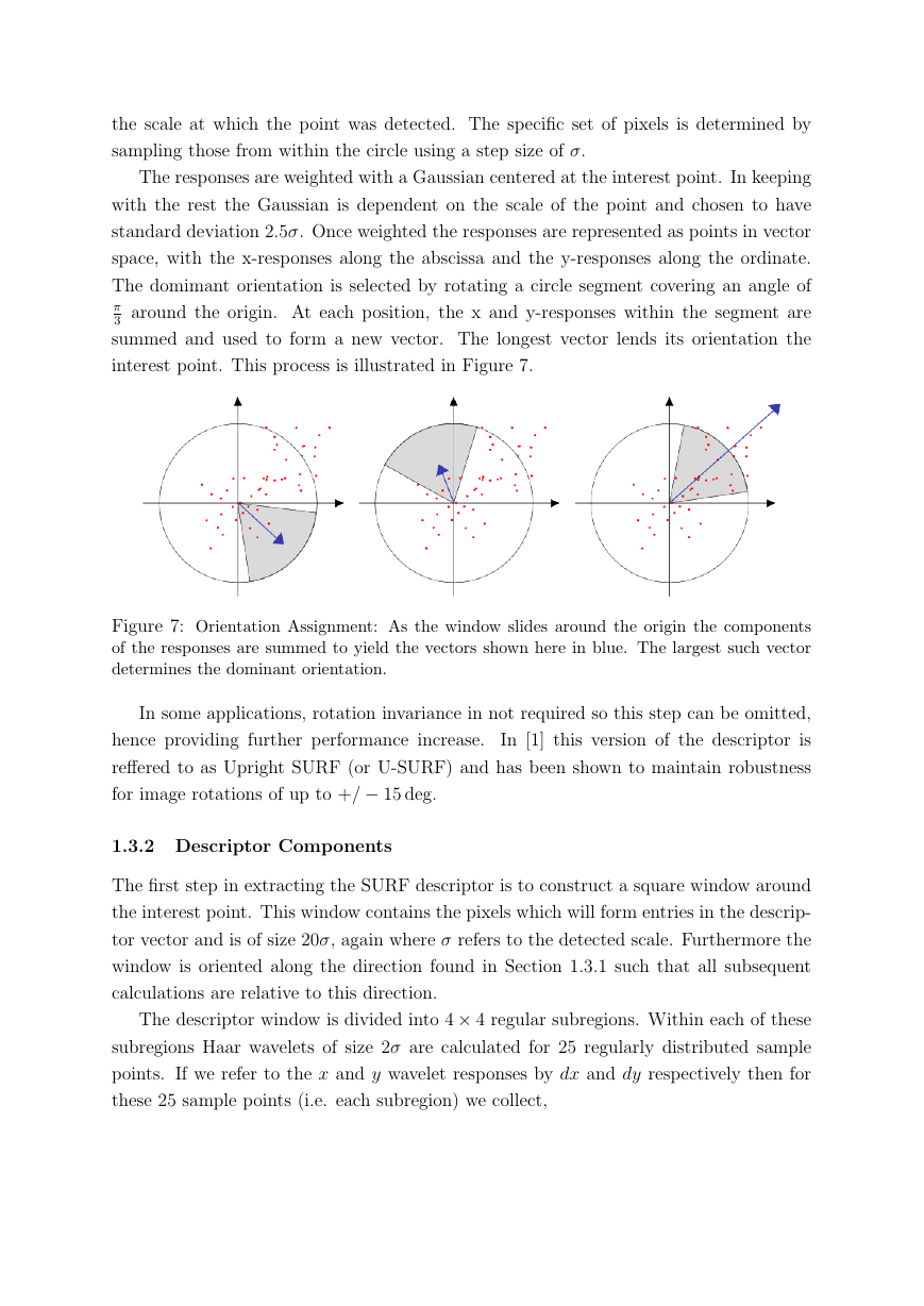
standard deviation 2.5σ. Once weighted the responses are represented as points in vector
space, with the x-responses along the abscissa and the y-responses along the ordinate.
The domimant orientation is selected by rotating a circle segment covering an angle of
π
3 around the origin. At each position, the x and y-responses within the segment are
summed and used to form a new vector. The longest vector lends its orientation the
interest point. This process is illustrated in Figure 7.
Figure 7: Orientation Assignment: As the window slides around the origin the components
of the responses are summed to yield the vectors shown here in blue. The largest such vector
determines the dominant orientation.
In some applications, rotation invariance in not required so this step can be omitted,
In [1] this version of the descriptor is
hence providing further performance increase.
reffered to as Upright SURF (or U-SURF) and has been shown to maintain robustness
for image rotations of up to +/ − 15 deg.
1.3.2 Descriptor Components
The first step in extracting the SURF descriptor is to construct a square window around
the interest point. This window contains the pixels which will form entries in the descrip-
tor vector and is of size 20σ, again where σ refers to the detected scale. Furthermore the
window is oriented along the direction found in Section 1.3.1 such that all subsequent
calculations are relative to this direction.
The descriptor window is divided into 4 × 4 regular subregions. Within each of these
subregions Haar wavelets of size 2σ are calculated for 25 regularly distributed sample
points. If we refer to the x and y wavelet responses by dx and dy respectively then for
these 25 sample points (i.e. each subregion) we collect,
�


 2023年江西萍乡中考道德与法治真题及答案.doc
 2012年重庆南川中考生物真题及答案.doc
 2013年江西师范大学地理学综合及文艺理论基础考研真题.doc
 2020年四川甘孜小升初语文真题及答案I卷.doc
 2020年注册岩土工程师专业基础考试真题及答案.doc
 2023-2024学年福建省厦门市九年级上学期数学月考试题及答案.doc
 2021-2022学年辽宁省沈阳市大东区九年级上学期语文期末试题及答案.doc
 2022-2023学年北京东城区初三第一学期物理期末试卷及答案.doc
 2018上半年江西教师资格初中地理学科知识与教学能力真题及答案.doc
 2012年河北国家公务员申论考试真题及答案-省级.doc
 2020-2021学年江苏省扬州市江都区邵樊片九年级上学期数学第一次质量检测试题及答案.doc
 2022下半年黑龙江教师资格证中学综合素质真题及答案.doc