Variational Mode Decomposition.pdf

发布时间：2022-05-31 发布人：admin 分类：说明书资料大小：5.38M 资料格式：pdf 举报版权申诉

qq_44143405-12361446-16359647266824571714.pdf-第1页.png

第1页 / 共15页

qq_44143405-12361446-16359647266824571714.pdf-第2页.png

第2页 / 共15页

qq_44143405-12361446-16359647266824571714.pdf-第3页.png

第3页 / 共15页

qq_44143405-12361446-16359647266824571714.pdf-第4页.png

第4页 / 共15页

qq_44143405-12361446-16359647266824571714.pdf-第5页.png

第5页 / 共15页

qq_44143405-12361446-16359647266824571714.pdf-第6页.png

第6页 / 共15页

qq_44143405-12361446-16359647266824571714.pdf-第7页.png

第7页 / 共15页

qq_44143405-12361446-16359647266824571714.pdf-第8页.png

第8页 / 共15页

文本预览

This article has been accepted for publication in a future issue of this journal, but has not been fully edited. Content may change prior to final publication. Citation information: DOI 10.1109/TSP.2013.2288675, IEEE Transactions on Signal Processing IEEE TRANSACTIONS ON SIGNAL PROCESSING, VOL. X, NO. Y, ZZZ 20WW 1 Variational Mode Decomposition Konstantin Dragomiretskiy and Dominique Zosso∗, Member, IEEE Abstract—In the late nineties, Huang introduced the algorithm called Empirical Mode Decomposition, which is widely used today to recursively decompose a signal into different modes of unknown but separate spectral bands. EMD is known for lim- itations like sensitivity to noise and sampling, These limitations could only partially be addressed by more mathematical attempts to this decomposition problem, like synchrosqueezing, empirical wavelets or recursive variational decomposition. Here, we propose an entirely non-recursive variational mode decomposition model, where the modes are extracted concur- rently. The model looks for an ensemble of modes and their respective center frequencies, such that the modes collectively reproduce the input signal, while each being smooth after demodulation into baseband. In Fourier domain, this corresponds to a narrow-band prior. We show important relations to Wiener ﬁlter denoising. Indeed, the proposed method is a generalization of the classic Wiener ﬁlter into multiple, adaptive bands. Our model provides a solution to the decomposition problem that is theoretically well founded and still easy to understand. The variational model is efﬁciently optimized using an alternating direction method of multipliers approach. Preliminary results show attractive performance with respect to existing mode decomposition models. In particular, our proposed model is much more robust to sampling and noise. Finally, we show promising practical decomposition results on a series of artiﬁcial and real data. Index Terms—Mode decomposition, variational problem, Wiener ﬁlter, AM-FM, spectral decomposition, Hilbert trans- form, Fourier transform, augmented Lagrangian. I. INTRODUCTION E MPIRICAL MODE DECOMPOSITON (EMD) proposed by Huang et al. [1] is an algorithmic method to detect and decompose a signal into principal “modes”. This algorithm recursively detects local minima/maxima in a signal, estimates lower/upper envelopes by interpolation of these extrema, re- moves the average of the envelopes as “low-pass” centerline, thus isolating the high-frequency oscillations as “mode” of a signal, and continues recursively on the remaining “low- pass” centerline. In some cases, this sifting algorithm does indeed decompose a signal into principal modes, however the resulting decomposition is highly dependent on methods of extremal point ﬁnding, interpolation of extremal points into carrier envelopes, and the stopping criteria imposed. The lack of mathematical theory and the aformentioned degrees of Copyright c 2013 IEEE. Personal use of this material is permitted. However, permission to use this material for any other purposes must be obtained from the IEEE by sending a request to pubs-persmissions@ieee.org. ∗ To whom correspondence should be addressed. This work is supported by the Swiss National Science Foundation (SNF) under grants PBELP2 137727 and P300P2 147778, the W. M. Keck Foundation, ONR grants N000141210838 and N000141210040, and NSF grant DMS- 1118971. The authors are with the Department of Mathematics, University of California, Los Angeles (UCLA), Box 951555, Los Angeles, CA 90095-1555, USA, {konstantin,zosso}@math.ucla.edu. 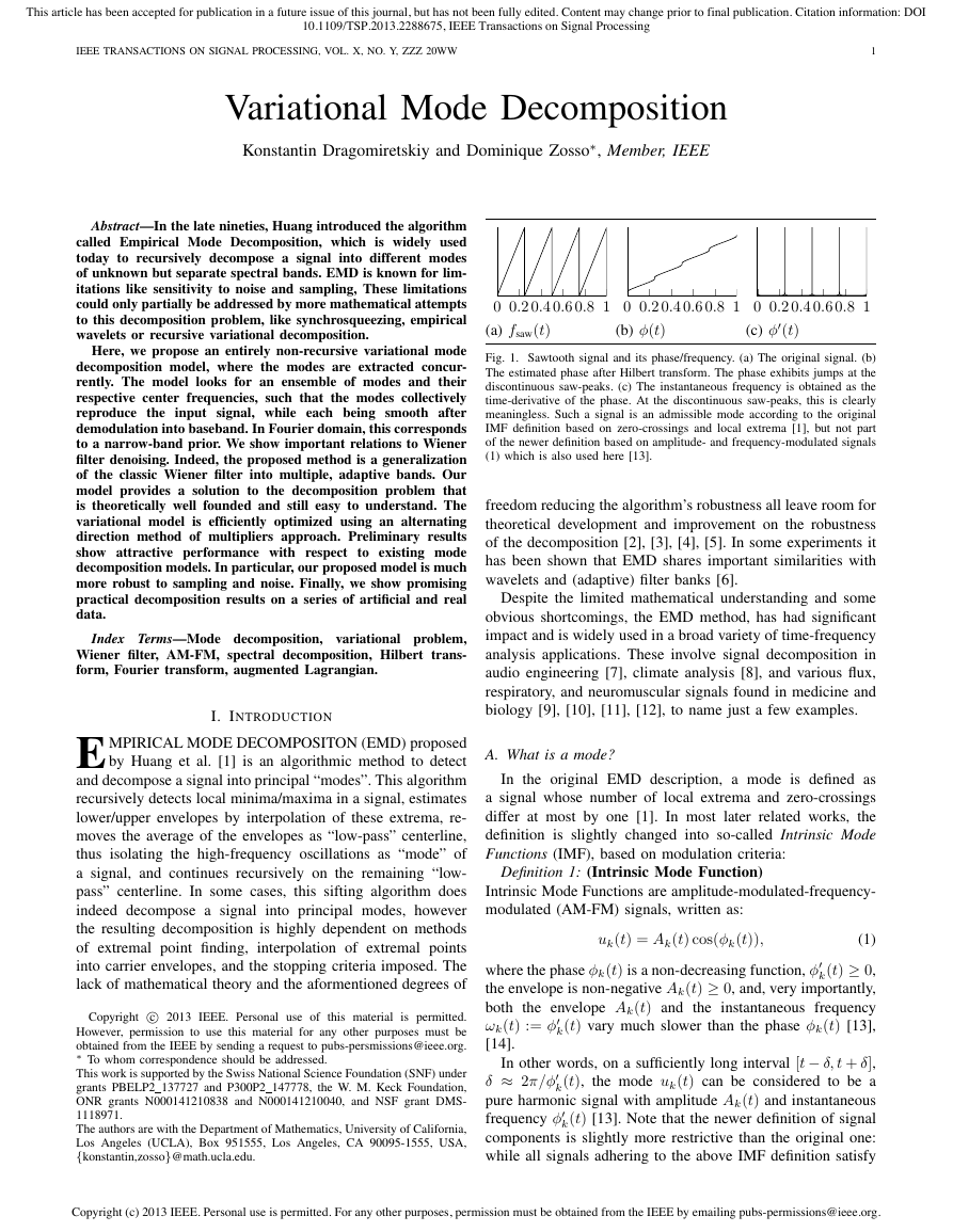0 0.2 0.4 0.6 0.8 1 0 0.2 0.4 0.6 0.8 1 0 0.2 0.4 0.6 0.8 1 (a) fsaw(t) (c) φ(t) (b) φ(t) Fig. 1. Sawtooth signal and its phase/frequency. (a) The original signal. (b) The estimated phase after Hilbert transform. The phase exhibits jumps at the discontinuous saw-peaks. (c) The instantaneous frequency is obtained as the time-derivative of the phase. At the discontinuous saw-peaks, this is clearly meaningless. Such a signal is an admissible mode according to the original IMF deﬁnition based on zero-crossings and local extrema [1], but not part of the newer deﬁnition based on amplitude- and frequency-modulated signals (1) which is also used here [13]. freedom reducing the algorithm’s robustness all leave room for theoretical development and improvement on the robustness of the decomposition [2], [3], [4], [5]. In some experiments it has been shown that EMD shares important similarities with wavelets and (adaptive) ﬁlter banks [6]. Despite the limited mathematical understanding and some obvious shortcomings, the EMD method, has had signiﬁcant impact and is widely used in a broad variety of time-frequency analysis applications. These involve signal decomposition in audio engineering [7], climate analysis [8], and various ﬂux, respiratory, and neuromuscular signals found in medicine and biology [9], [10], [11], [12], to name just a few examples. A. What is a mode? In the original EMD description, a mode is deﬁned as a signal whose number of local extrema and zero-crossings differ at most by one [1]. In most later related works, the deﬁnition is slightly changed into so-called Intrinsic Mode Functions (IMF), based on modulation criteria: Deﬁnition 1: (Intrinsic Mode Function) Intrinsic Mode Functions are amplitude-modulated-frequency- modulated (AM-FM) signals, written as: uk(t) = Ak(t) cos(φk(t)), (1) k(t) ≥ 0, where the phase φk(t) is a non-decreasing function, φ the envelope is non-negative Ak(t) ≥ 0, and, very importantly, both the envelope Ak(t) and the instantaneous frequency ωk(t) := φ k(t) vary much slower than the phase φk(t) [13], [14]. In other words, on a sufﬁciently long interval [t − δ, t + δ], δ ≈ 2π/φ k(t), the mode uk(t) can be considered to be a pure harmonic signal with amplitude Ak(t) and instantaneous frequency φ k(t) [13]. Note that the newer deﬁnition of signal components is slightly more restrictive than the original one: while all signals adhering to the above IMF deﬁnition satisfy Copyright (c) 2013 IEEE. Personal use is permitted. For any other purposes, permission must be obtained from the IEEE by emailing pubs-permissions@ieee.org.

This article has been accepted for publication in a future issue of this journal, but has not been fully edited. Content may change prior to final publication. Citation information: DOI 10.1109/TSP.2013.2288675, IEEE Transactions on Signal Processing 2 IEEE TRANSACTIONS ON SIGNAL PROCESSING, VOL. X, NO. Y, ZZZ 20WW 0 0.2 0.4 0.6 0.8 1 101 (a) AM signal and spectrum. (∆f = 0) 0 0.2 0.4 0.6 0.8 1 101 (b) FM signal and spectrum. (fFM ∆f ) 0 0.2 0.4 0.6 0.8 1 101 (c) FM signal and spectrum. (fFM ∆f ) 102 103 102 103 102 103 103 102 101 100 103 102 101 100 103 102 101 100 103 102 101 100 1 0 −1 1 0.5 0 −0.5 −1 1 0.5 0 −0.5 −1 1 0 −1 the original EMD mode properties, the converse is not nec- essarily true [13]. The immediate consequence of the newer IMF deﬁnition, however, is limited bandwidth, as we show in the next paragraphs, and which is the central assumption that allows mode separation in the proposed variational mode decomposition model. Our restricted class of admissible mode functions is also motivated by analysis in [3], for they are well-behaved with respect to time-frequency analysis of ex- tracted modes, as routinely performed in the Hilbert-Huang- Transform [1]. In contrast, the original IMF deﬁnition also admits non-C 1 and discontinuous signals like the sawtooth, for which the estimated instantaneous frequency is not physically meaningful, see Fig. 1. Indeed, if ωk is the mean frequency of a mode, then its practical bandwidth increases both with the maximum deviation ∆f of the instantaneous frequency from its center (carrier frequency, fc), and with the rate of this excursion, fFM, according to Carson’s rule1 [15]: BWFM = 2(∆f + fFM). (2) In addition to this, the bandwidth of the envelope Ak(t) modulating the amplitude of the FM signal, itself given by its highest frequency fAM, broadens the spectrum even further: Deﬁnition 2: (Total practical IMF bandwidth) We estimate the total practical bandwidth of an IMF as BWAM-FM = 2(∆f + fFM + fAM). 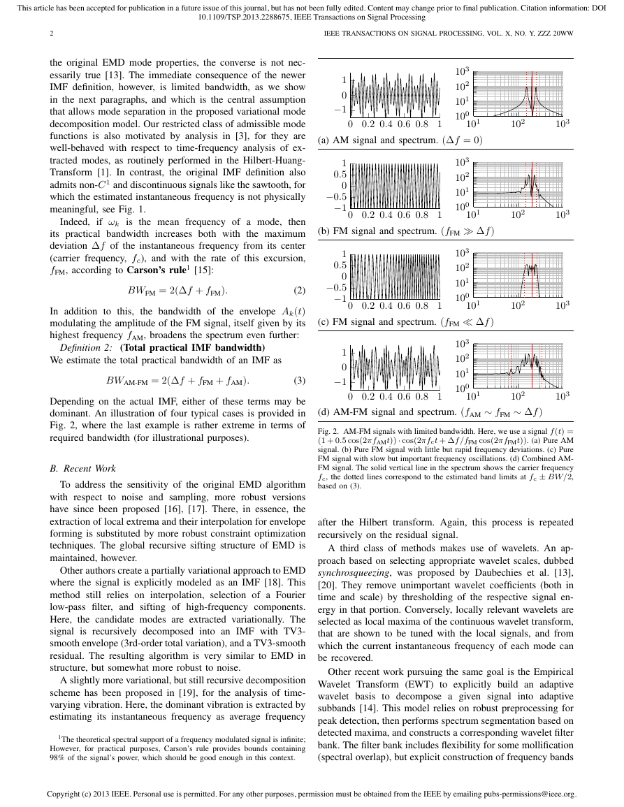(3) Depending on the actual IMF, either of these terms may be dominant. An illustration of four typical cases is provided in Fig. 2, where the last example is rather extreme in terms of required bandwidth (for illustrational purposes). B. Recent Work To address the sensitivity of the original EMD algorithm with respect to noise and sampling, more robust versions have since been proposed [16], [17]. There, in essence, the extraction of local extrema and their interpolation for envelope forming is substituted by more robust constraint optimization techniques. The global recursive sifting structure of EMD is maintained, however. Other authors create a partially variational approach to EMD where the signal is explicitly modeled as an IMF [18]. This method still relies on interpolation, selection of a Fourier low-pass ﬁlter, and sifting of high-frequency components. Here, the candidate modes are extracted variationally. The signal is recursively decomposed into an IMF with TV3- smooth envelope (3rd-order total variation), and a TV3-smooth residual. The resulting algorithm is very similar to EMD in structure, but somewhat more robust to noise. A slightly more variational, but still recursive decomposition scheme has been proposed in [19], for the analysis of time- varying vibration. Here, the dominant vibration is extracted by estimating its instantaneous frequency as average frequency 1The theoretical spectral support of a frequency modulated signal is inﬁnite; However, for practical purposes, Carson’s rule provides bounds containing 98% of the signal’s power, which should be good enough in this context. 0 0.2 0.4 0.6 0.8 1 101 102 103 (d) AM-FM signal and spectrum. (fAM ∼ fFM ∼ ∆f ) Fig. 2. AM-FM signals with limited bandwidth. Here, we use a signal f (t) = (1 + 0.5 cos(2πfAMt)) · cos(2πfct + ∆f /fFM cos(2πfFMt)). (a) Pure AM signal. (b) Pure FM signal with little but rapid frequency deviations. (c) Pure FM signal with slow but important frequency oscillations. (d) Combined AM- FM signal. The solid vertical line in the spectrum shows the carrier frequency fc, the dotted lines correspond to the estimated band limits at fc ± BW/2, based on (3). after the Hilbert transform. Again, this process is repeated recursively on the residual signal. A third class of methods makes use of wavelets. An ap- proach based on selecting appropriate wavelet scales, dubbed synchrosqueezing, was proposed by Daubechies et al. [13], [20]. They remove unimportant wavelet coefﬁcients (both in time and scale) by thresholding of the respective signal en- ergy in that portion. Conversely, locally relevant wavelets are selected as local maxima of the continuous wavelet transform, that are shown to be tuned with the local signals, and from which the current instantaneous frequency of each mode can be recovered. Other recent work pursuing the same goal is the Empirical Wavelet Transform (EWT) to explicitly build an adaptive wavelet basis to decompose a given signal into adaptive subbands [14]. This model relies on robust preprocessing for peak detection, then performs spectrum segmentation based on detected maxima, and constructs a corresponding wavelet ﬁlter bank. The ﬁlter bank includes ﬂexibility for some molliﬁcation (spectral overlap), but explicit construction of frequency bands Copyright (c) 2013 IEEE. Personal use is permitted. For any other purposes, permission must be obtained from the IEEE by emailing pubs-permissions@ieee.org.

This article has been accepted for publication in a future issue of this journal, but has not been fully edited. Content may change prior to final publication. Citation information: DOI 10.1109/TSP.2013.2288675, IEEE Transactions on Signal Processing DRAGOMIRETSKIY AND ZOSSO: VARIATIONAL MODE DECOMPOSITION 3 still appears slightly strict. Finally, a related decomposition into different wavelet bands was suggested by [21]. The author introduces two complemen- tary wavelet bases with different Q-factor. This allows discrim- inating between sustained oscillations (high-resonance compo- nents), and non-oscillatory, short-term transients. Indeed, the high-resonance components can sparsely be represented in a high-Q wavelet basis, while transients will be synthesized by low-Q wavelets. C. Proposed method In this paper, we propose a new, fully intrinsic and adaptive, variational method, the minimization of which leads to a decomposition of a signal into its principal modes. Indeed, the current decomposition models are mostly limited by 1) their al- gorithmic ad-hoc nature lacking mathematical theory (EMD), 2) the recursive sifting in most methods, which does not allow for backward error correction, 3) the inability to properly cope with noise, 4) the hard band-limits of wavelet approaches, and 5) the requirement of predeﬁning ﬁlter bank boundaries in EWT. In contrast, we propose a variational model that determines the relevant bands adaptively, and estimates the corresponding modes concurrently, thus properly balancing errors between them. Motivated by the narrow-band properties corresponding to the current common IMF deﬁnition, we look for an ensemble of modes that reconstruct the given input signal optimally (either exactly, or in a least-squares sense), while each being band-limited about a center frequency estimated on-line. Here, our variational model speciﬁcally can address the presence of noise in the input signal. Indeed, the tight relations to the Wiener ﬁlter actually suggest that our approach has some optimality in dealing with noise. The variational model assesses the bandwidth of the modes as H 1-norm, after shifting the Hilbert-complemented, analytic signal down into baseband by complex harmonic mixing. The resulting optimization scheme is very simple and fast: each mode is iteratively updated directly in Fourier domain, as the narrow-band Wiener ﬁlter corresponding to the current estimate of the mode’s center-frequency being applied to the signal estimation residual of all other modes; then the center frequency is re-estimated as the center-of-gravity of the mode’s power spectrum. Our quantitative results on tone detection and separation show excellent performance irrespective of harmonic frequencies, in particular when compared to the apparent limits of EMD in this respect. Further, qualitative results on synthetic and real test signals are convincing, also regarding robustness to signal noise. The rest of this paper is organized as follows: Section II introduces the notions of the Wiener ﬁlter, the Hilbert transform, and the analytic signal. Also, we brieﬂy review the concept of frequency shifting through harmonic mixing. These concepts are the very building blocks of our variational mode decomposition model. Although signal processing scholars can be expected to be familiar with these concepts, we include this short refresher to keep the manuscript largely self-contained and accessible to readers of different provenience. Section III presents and explains our variational model in detail, our algorithm to minimize it, and ﬁner technicalities on opti- mization, boundaries and periodicity. Section IV contains our experiments and results, namely some simple quantitative per- formance evaluations, and comparisons to EMD, and various synthetic multi-mode signals and our method’s decomposition of them. Speciﬁcally, tone detection and separation, as well as noise robustness will be analyzed and compared to that of EMD. Additionally, real signals will be considered. Section V concludes on our proposed variational mode decomposi- tion method, summarizes again the main assumptions and limitations, and includes some future directions and expected improvements. II. TOOLS FROM SIGNAL PROCESSING In this section we brieﬂy review a few concepts and tools from signal processing that will constitute the building blocks of our variational mode decomposition model. First, we present a classical case of Wiener ﬁltering for denoising. Next, we describe the Hilbert transform and its use in the construction of a single-side band analytic signal. Finally, we show how multiplication with pure complex harmonics is used to shift the frequencies in a signal. A. Wiener ﬁltering Let us start with a simple denoising problem. Consider the observed signal f0(t), a copy of the original signal f (t) affected by additive zero-mean Gaussian noise: f0 = f + η (4) Recovering the unknown signal f is a typical ill-posed inverse problem [22], [23], classically addressed using Tikhonov reg- ularization [24], [25]: f − f02 min f 2 + α∂tf2 2 , (5) ˆf (ω) = 1 + αω2 , of which the Euler-Lagrange equations are easily obtained and typically solved in Fourier domain: ˆf0 (6) √ where ˆf (ω) := F{f (·)}(ω) := 1/ R f (t)e−jωtdt, with j2 = −1, is the Fourier transform of the signal f (t). Clearly, the recovered signal f is a low-pass narrow-band selection of the input signal f0 around ω = 0. Indeed, the solution corresponds to convolution with a Wiener ﬁlter, where α represents the variance of the white noise, and the signal has a lowpass 1/ω2 power spectrum prior [26], [27]. 2π B. Hilbert transform and analytic signal Here, we cite the deﬁnition of the Hilbert transform given in [28]: Deﬁnition 3: (Hilbert transform) The 1-D Hilbert transform is the linear, shift-invariant operator H that maps all 1-D cosine functions into their corresponding sine functions. It is an all-pass ﬁlter that is characterized by the transfer function ˆh(ω) = −j sgn(ω) = −jω/|ω|. Copyright (c) 2013 IEEE. Personal use is permitted. For any other purposes, permission must be obtained from the IEEE by emailing pubs-permissions@ieee.org.

This article has been accepted for publication in a future issue of this journal, but has not been fully edited. Content may change prior to final publication. Citation information: DOI 10.1109/TSP.2013.2288675, IEEE Transactions on Signal Processing 4 IEEE TRANSACTIONS ON SIGNAL PROCESSING, VOL. X, NO. Y, ZZZ 20WW Thus, the Hilbert transform is a multiplier operator in the spec- tral domain. The corresponding impulse response is h(t) = 1/(πt). Because convolution with h(t) is not integrable, the transform Hf (t) of a signal f (t) is obtained as Hilbert the Cauchy principal value (denoted p.v.) of the convolution integral: Hf (t) = 1 π p.v. f (v) t − v R dv. (7) For further properties and analysis of the Hilbert transform, we refer e.g. to [29]. The most prominent use of the Hilbert transform is in the construction of an analytic signal from a purely real signal, as proposed by Gabor [30]. Deﬁnition 4: (Analytic signal) Let f (t) be a purely real signal. The complex-valued analytic signal is now deﬁned as: fA(t) = f (t) + jHf (t) = A(t)ejφ(t). (8) This analytic signal has the following important properties. The complex exponential term ejφ(t) is a phasor describing the rotation of the complex signal in time, φ(t) being the phase, while the amplitude is governed by the real envelope A(t). This representation is particularly useful in the analysis of time-varying amplitude and instantaneous frequency, deﬁned as ω(t) = dφ(t)/dt. In particular for IMF signals of the form (1), where the amplitude Ak changes slowly enough, Bedrosian’s theorem applies [31], and the analytic signal directly inherits the same amplitude function: uk,A(t) = Ak(t) (cos(φ(t)) + j sin(φ(t))) = Ak(t)ejφ(t). (9) The second property is the unilateral spectrum of the analytic signal, consisting only of non-negative frequencies. Finally, we note that from such an analytic signal, the original (real) signal is easily retrieved as the real part: f (t) = {fA(t)}. (10) C. Frequency mixing and heterodyne demodulation The last concept that we wish to recall before introducing the proposed variational mode decomposition, is the principle of frequency mixing. Mixing is the process of combining two signals non-linearily, thus introducing cross-frequency terms in the output. The simplest mixer is multiplication. Multiplying two real signals with frequencies ω1 and ω2, respectively, creates mixed frequencies in the output at ω1−ω2 and ω1 +ω2, which is easily illustrated by the following trigonometric identity: 2 cos(ω1t) cos(ω2t) = cos((ω1 + ω2)t) + cos((ω1 − ω2)t). (11) Here we mix the two respective analytic signals: ejω1tejω2t = ej(ω1+ω2)t, (12) and thus, is automatically “mono-tone” (constituted of a single frequency only). In Fourier terms, this is well known as the following transform pair: the mixed signal fA(t)e−jω0t F←→ ˆfA(ω) ∗ δ(ω + ω0) = ˆfA(ω + ω0), (13) where δ is the Dirac distribution and ∗ denotes convolution. Thus, multiplying an analytic signal with a pure exponential results in simple frequency shifting. III. VARIATIONAL MODE DECOMPOSITION In this section we introduce our proposed model for vari- ational mode decomposition, essentially based on the three concepts outlined in the previous section. The goal of VMD is to decompose a real valued input signal f into a discrete number of sub-signals (modes), uk, that have speciﬁc sparsity properties while reproducing the input2. Here, the sparsity prior of each mode is chosen to be its bandwidth in spectral domain. In other words, we assume each mode k to be mostly compact around a center pulsation ωk, which is to be determined along with the decomposition. In order to assess the bandwidth of a mode, we propose the following scheme: 1) for each mode uk, compute the associated analytic signal by means of the Hilbert transform in order to obtain a unilateral frequency spectrum. 2) for each mode, shift the mode’s frequency spectrum to “baseband”, by mixing with an exponential tuned to the respective estimated center frequency. 3) The bandwidth is now estimated through the H 1 Gaussian smoothness of the demodulated signal, i.e. the squared L2-norm of the gradient. The resulting constrained variational problem is the following: k ∂t δ(t) + j πt min {uk},{ωk} 2 2 e−jωkt uk = f (14) ∗ uk(t) s.t. k :=K k frequencies, respectively. Equally, where {uk} := {u1, . . . , uK} and {ωk} := {ω1, . . . , ωK} are shorthand notations for the set of all modes and their center k=1 is understood as the summation over all modes. The reconstruction constraint can be addressed in different ways. Here, we suggest making use of both a quadratic penalty term and Lagrangian multipliers, λ, in order to render the problem unconstrained. The quadratic penalty is a classic way to encourage reconstruction ﬁdelity, typically in the presence of additive i.i.d. Gaussian noise. The weight of the penalty term is derived from such a Bayesian prior to be inversely proportional to the noise level in the data. Conversely, in a noisefree setting, the weight needs to be inﬁnitely big in order to enforce strict data ﬁdelity, rendering the system ill- conditioned in the process. On the other hand, Lagrangian multipliers are a common way of enforcing constraints strictly. The combination of the two terms thus beneﬁts both from the nice convergence properties of the quadratic penalty at ﬁnite weight, and the strict enforcement of the constraint by the Lagrangian multiplier. Therefore, we introduce the augmented 2For the sake of completeness, we require that both signal and modes are integrable, and square integrable upto second derivatives: f, uk ∈ L1∩W 2,2. We call this functional space X for further reference. This ensures that later integrals are ﬁnite, and that Fourier isometry applies. In practice, we will deal with discrete signals and in our implementations the solutions are tacitly discretized. Copyright (c) 2013 IEEE. Personal use is permitted. For any other purposes, permission must be obtained from the IEEE by emailing pubs-permissions@ieee.org.

This article has been accepted for publication in a future issue of this journal, but has not been fully edited. Content may change prior to final publication. Citation information: DOI 10.1109/TSP.2013.2288675, IEEE Transactions on Signal Processing 6 IEEE TRANSACTIONS ON SIGNAL PROCESSING, VOL. X, NO. Y, ZZZ 20WW is the frequency of a least squares linear regression to the instantaneous phase observed in the mode. Plugging the solutions of the sub-optimizations into the ADMM algorithm 1, and directly optimizing in Fourier do- main where appropriate, we get the complete algorithm for variational mode decomposition, summarized in algorithm 2. Algorithm 2 Complete optimization of VMD k}, ˆλ1, n ← 0 k}, {ω1 Initialize {ˆu1 repeat n ← n + 1 for k = 1 : K do (ω) ← ˆf (ω) − Update ˆuk for all ω ≥ 0: ik ˆun 1 + 2α(ω − ωn k )2 i (ω) + ˆλn(ω) 2 (27) (28) Update ωk: k ← ωn+1 (ω)|2dω (ω)|2dω k ∞ ∞ 0 ω|ˆun+1 |ˆun+1 k 0 end for Dual ascent for all ω ≥ 0: ˆλn+1(ω) ← ˆλn(ω) + τ ˆf (ω) − ˆun+1 k (ω) (29) until convergence: k k ˆun+1 k − ˆun k2 2/ˆun k2 2 < . C. Exact reconstruction versus denoising Here, the role of the Lagrangian multiplier is to enforce the constraint, while the quadratic penalty improves convergence. If exact reconstruction is not the goal, in particular in the presence of (strong) noise that should not be included in the decomposition, using the quadratic penalty only while dropping the Lagrangian multiplier would be the appropriate choice. Indeed, the quadratic penalty on its own represents the least-squares data ﬁdelity prior associated with additive Gaussian noise. The Lagrangian multiplier is effectively shut- off by keeping its value at 0, most easily by simply choosing its update parameter τ = 0. D. On boundaries and periodicity Up until now, the signals f and the modes uk have been considered continuous over the whole axis t ∈ R. However, in signal processing we are much more likely to be working with signals that are both ﬁnite in time and resolution. Let us say we restrict the time window to t ∈ [0, 1]. The results presented so far equally hold for discrete, ﬁnite time signals, where simply the continuous Fourier transform is replaced by its discrete counterpart. The only problems arise at the boundaries of the signal. Indeed, when considering short-time signals, the implicit assumption here is that the signal considered is just a one- period extract of an inﬁnitely long, periodic signal. Conse- quently, the spectrum of a seemingly simple “general trend”- function on a short interval, say f : [0, 1] → R : f (t) = t, contains an important amount of high-frequency harmonics, since we are effectively looking at the spectrum of the periodic sawtooth function. Conversely in time domain, we realize that at the endpoints of the domain, the periodized function is discontinuous, thus severely affecting the H 1 smoothing term. There are several possible remedies to this. Ideally, one should exclude the boundaries of the domain in the evaluation of the smoothness, i.e. restrict its evaluation to the open inter- val (0, 1). However, this clearly breaks the Parseval/Plancherel Fourier isometry and the whole beauty of the spectral solution is lost. Here, the boundary issues can most easily be remedied by simple mirror extension of the signal by half its length on each side, effectively corresponding to Neumann boundary conditions, namely vanishing derivatives at the time domain boundaries. We will brieﬂy discuss an alternative for short- time analysis of non-stationary signals in the last section of this paper. IV. EXPERIMENTS AND RESULTS In this section, we apply the proposed VMD algorithm to a series of test signals in order to assess the validity of our approach. First, we focus on a few problems that have been successfully employed for highlighting the strengths and shortcomings of EMD, namely tones versus sampling, and tones separation [2]. Then we brieﬂy investigate noise robustness of VMD, sensitivity to initialization and over- and underbinning (choice of K). Finally, we shift our attention to more complex signals, which have already been used for evaluation in [18] and [14]. A. Tones and sampling When the input signal f = fν(t) = cos(2πνt) is composed of a pure harmonic, then the mode decomposition is expected to output exactly this harmonic. As reported in [2], [5], this does not happen to be the case with EMD, since the local extrema can suffer from important jittering with increasing frequency. In [2], the relative error e(ν) = fν(t) − u1(t)2/fν(t)2 (30) was introduced, and a quadratic increase with frequency of an upper bound to this relative error was reported for EMD. Further, EMD has pronounced spikes of near-perfect recon- struction when the sampling frequency is an even multiple of the tone’s frequency. 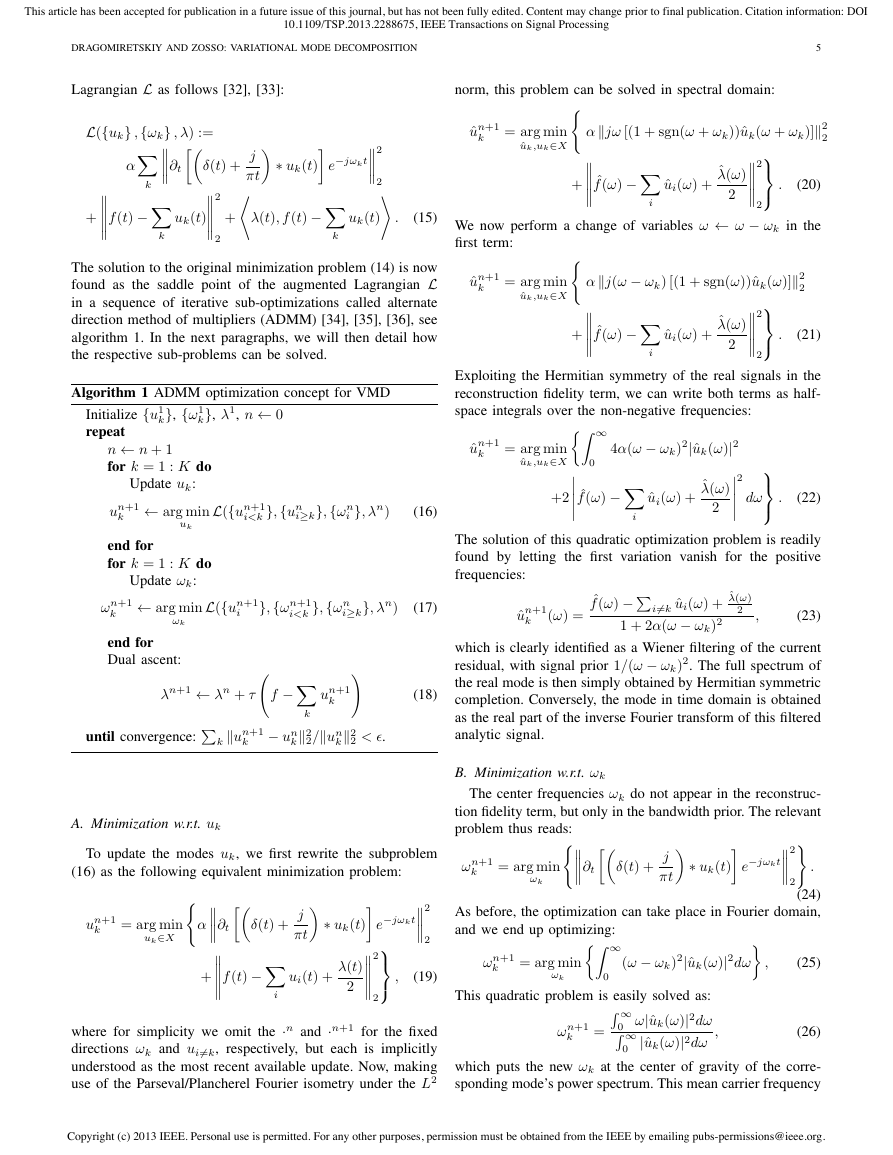Here, we perform this analysis for the proposed VMD model. The results for different convergence tolerance levels are shown in Fig. 3. It can be clearly seen that the relative reconstruction error is largely independent of the harmonic’s frequency. Moreover, the relative error is nicely controlled by the tolerance level . Copyright (c) 2013 IEEE. Personal use is permitted. For any other purposes, permission must be obtained from the IEEE by emailing pubs-permissions@ieee.org.

This article has been accepted for publication in a future issue of this journal, but has not been fully edited. Content may change prior to final publication. Citation information: DOI 10.1109/TSP.2013.2288675, IEEE Transactions on Signal Processing DRAGOMIRETSKIY AND ZOSSO: VARIATIONAL MODE DECOMPOSITION 7 100 10−3 10−6 10−2 (a) = 1e − 3 10−1 100 10−3 10−6 10−2 (b) = 1e − 5 10−1 100 10−3 10−6 100 10−3 10−6 10−1 10−1 10−2 (d) = 1e − 9 10−2 (c) = 1e − 7 Fig. 3. Mode decomposition of a pure harmonic. (a)–(d) Relative error for a range of 257 frequencies, for different convergence tolerance levels . The relative error does not correlate with the tone frequency. Further, reconstruction error can be controlled by decreasing the stopping criterion’s convergence tolerance, except for frequencies very close to the Nyquist frequency. In contrast, EMD’s relative tone reconstruction error is bounded by a quadratic increase with frequency (dotted line) [2]. 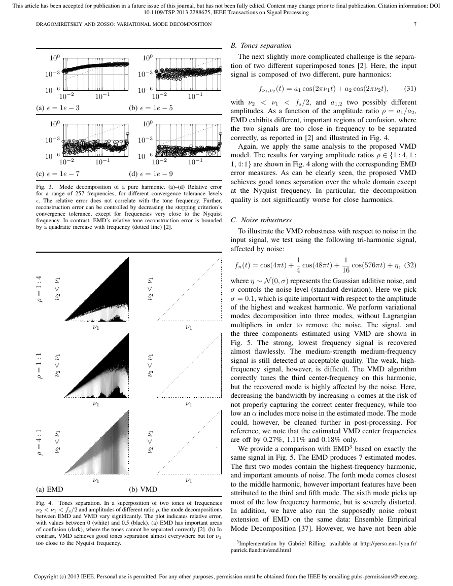4 : 1 = ρ 1 ν < 2 ν 1 : 1 = ρ 1 ν < 2 ν 1 : 4 = ρ 1 ν < 2 ν ν1 ν1 ν1 1 ν < 2 ν 1 ν < 2 ν 1 ν < 2 ν ν1 ν1 ν1 (a) EMD (b) VMD Fig. 4. Tones separation. In a superposition of two tones of frequencies ν2 < ν1 < fs/2 and amplitudes of different ratio ρ, the mode decompositions between EMD and VMD vary signiﬁcantly. The plot indicates relative error, with values between 0 (white) and 0.5 (black). (a) EMD has important areas of confusion (dark), where the tones cannot be separated correctly [2]. (b) In contrast, VMD achieves good tones separation almost everywhere but for ν1 too close to the Nyquist frequency. B. Tones separation The next slightly more complicated challenge is the separa- tion of two different superimposed tones [2]. Here, the input signal is composed of two different, pure harmonics: fν1,ν2 (t) = a1 cos(2πν1t) + a2 cos(2πν2t), (31) with ν2 < ν1 < fs/2, and a1,2 two possibly different amplitudes. As a function of the amplitude ratio ρ = a1/a2, EMD exhibits different, important regions of confusion, where the two signals are too close in frequency to be separated correctly, as reported in [2] and illustrated in Fig. 4. Again, we apply the same analysis to the proposed VMD model. The results for varying amplitude ratios ρ ∈ {1 : 4, 1 : 1, 4:1} are shown in Fig. 4 along with the corresponding EMD error measures. As can be clearly seen, the proposed VMD achieves good tones separation over the whole domain except at the decomposition quality is not signiﬁcantly worse for close harmonics. the Nyquist frequency. In particular, C. Noise robustness To illustrate the VMD robustness with respect to noise in the input signal, we test using the following tri-harmonic signal, affected by noise: 1 4 1 16 cos(48πt) + cos(576πt) + η, (32) fn(t) = cos(4πt) + where η ∼ N (0, σ) represents the Gaussian additive noise, and σ controls the noise level (standard deviation). Here we pick σ = 0.1, which is quite important with respect to the amplitude of the highest and weakest harmonic. We perform variational modes decomposition into three modes, without Lagrangian multipliers in order to remove the noise. The signal, and the three components estimated using VMD are shown in Fig. 5. The strong, is recovered almost ﬂawlessly. The medium-strength medium-frequency signal is still detected at acceptable quality. The weak, high- frequency signal, however, is difﬁcult. The VMD algorithm correctly tunes the third center-frequency on this harmonic, but the recovered mode is highly affected by the noise. Here, decreasing the bandwidth by increasing α comes at the risk of not properly capturing the correct center frequency, while too low an α includes more noise in the estimated mode. The mode could, however, be cleaned further in post-processing. For reference, we note that the estimated VMD center frequencies are off by 0.27%, 1.11% and 0.18% only. lowest frequency signal We provide a comparison with EMD3 based on exactly the same signal in Fig. 5. The EMD produces 7 estimated modes. The ﬁrst two modes contain the highest-frequency harmonic, and important amounts of noise. The forth mode comes closest to the middle harmonic, however important features have been attributed to the third and ﬁfth mode. The sixth mode picks up most of the low frequency harmonic, but is severely distorted. In addition, we have also run the supposedly noise robust extension of EMD on the same data: Ensemble Empirical Mode Decomposition [37]. However, we have not been able 3Implementation by Gabriel Rilling, available at http://perso.ens-lyon.fr/ patrick.ﬂandrin/emd.html Copyright (c) 2013 IEEE. Personal use is permitted. For any other purposes, permission must be obtained from the IEEE by emailing pubs-permissions@ieee.org.

This article has been accepted for publication in a future issue of this journal, but has not been fully edited. Content may change prior to final publication. Citation information: DOI 10.1109/TSP.2013.2288675, IEEE Transactions on Signal Processing 8 1 0 −1 1 0 −1 0 0.2 0.4 0.6 0.8 1 0 0.2 0.4 0.6 0.8 1 (a) fn(t) 0.4 0.2 0 −0.2 0 0.2 0.4 0.6 0.8 1 (b) VMD uk(t) 0.1 0 −0.1 −0.2 0 0.2 0.4 0.6 0.8 1 104 101 10−2 (c) | ˆfn|(ω) 101 104 101 10−2 101 (d) |ˆuk|(ω) 102 103 102 103 0.2 0.1 0 −0.1 −0.2 0.4 0.2 0 −0.2 −0.4 1 0.5 0 −0.5 −1 0 0.2 0.4 0.6 0.8 1 0 0.2 0.4 0.6 0.8 1 0 0.2 0.4 0.6 0.8 1 0.2 0 −0.2 0.4 0.2 0 −0.2 −0.4 0.5 0 −0.5 0.2 0.1 0 −0.1 0 0.2 0.4 0.6 0.8 1 0 0.2 0.4 0.6 0.8 1 0 0.2 0.4 0.6 0.8 1 0 0.2 0.4 0.6 0.8 1 (e) EMD uk(t) Fig. 5. Decomposition of noisy tri-harmonic. (a) The noisy input signal. (b) The three modes extracted by denoising VMD (inactive Lagrangian multiplier), and the theoretical mode (dotted). (c) The spectrum of the input signal (expected mode-frequencies as vertical dashed lines), and (d) its distribution over the three modes. (e) The 7 components extracted by EMD. None of the modes corresponds to a pure harmonic. IEEE TRANSACTIONS ON SIGNAL PROCESSING, VOL. X, NO. Y, ZZZ 20WW to achieve signiﬁcantly better results than the ones produced by traditional EMD. D. Initialization and convergence Although we cannot provide a detailed convergence analysis in the scope of the present paper, we do wish to comment on some convergence properties and sensitivity to initial conditions. We propose to illustrate the algorithm success for varying random initializations of the center frequencies, the rest of the variables being essentially updated from there. Indeed, the proposed algorithm is not guaranteed to con- verge to a global minimum. Therefore, the result does depend on the initialization, and in particular the success rate depends on the noise level. For sufﬁciently low noise levels, the La- grangian multiplier can be used to enforce exact reconstruction of the input signal. Therefore, even with unfortunate initializa- tion leading to “duplicate and forgotten modes”, the forgotten modes will be picked up eventually. In Fig. 6(a) we show the 100 trajectories of randomly initialized center frequencies for the noisy triharmonic (32), at low noise level σ = 0.005, and with Lagrangian multipliers active. In this setting, we were 100% successful. The success rate for bigger σ is shown in Fig. 6(c), where one clearly sees the impact of Lagrangian multipliers: They’re presence ensures optimal convergence at low noise level, but becomes a strict impediment if noise becomes more important. In the presence of stronger noise, the Lagrangian multipliers are not useful anymore, since we wish to eliminate the noise from the estimated modes. Here, convergence is more sensitive to noise, and the success rate for the noisy triharmonic (32) drops. A detailed curve of the success rate as a function of the noise level σ is shown in Fig. 6(b). Interestingly, some amount of noise is beneﬁcial with regards to ﬁnding the correct center frequencies. Like the non-zero temperature in simulated annealing [38], [39], some noise in the data ﬂattens the spectra and helps the algorithm evolve out of wrong local minima. This leads to maximum success rate of about 90- 95% between σ = 0.02 and 0.08. Above, the noise starts masking the weakest harmonic and the success rate falls off. The successful trajectories are typically characterized by fast convergence, compared to the failing runs. Also, at σ = 0.1 for example, all initializations within 14.39 ≤ ω2 ≤ 1050, and within 743 ≤ ω3 ≤ 2556 were successful, which means that in this difﬁcult example even the weakest component need only be initialized with an error less than 40% for successful segmentation. This does not seem very strict for a practical application where some prior knowledge about the expected oscillations is available. E. Over- and undersegmentation, uniqueness A classical shortcoming of many segmentation algorithms is the need to tell in advance into how many clusters (or modes, in the present case), data are to be binned. This is no different with the proposed VMD algorithm. In order to study the effects of over- and underbinning the given data, we evaluate here the outcome of VMD using too few or too many modes, K. Copyright (c) 2013 IEEE. Personal use is permitted. For any other purposes, permission must be obtained from the IEEE by emailing pubs-permissions@ieee.org.

分享到：

赞收藏

资料库

Variational Mode Decomposition.pdf

相关推荐

人工智能

热门标签

最新资料