7
1
0
2
n
u
J
9
1
]
L
C
.
s
c
[
2
v
2
6
7
3
0
.
6
0
7
1
:
v
i
X
r
a
Attention Is All You Need
Ashish Vaswani∗
Google Brain
avaswani@google.com
Noam Shazeer∗
Google Brain
noam@google.com
Niki Parmar∗
Google Research
nikip@google.com
Jakob Uszkoreit∗
Google Research
usz@google.com
Llion Jones∗
Google Research
llion@google.com
Aidan N. Gomez∗†
University of Toronto
aidan@cs.toronto.edu
Łukasz Kaiser∗
Google Brain
lukaszkaiser@google.com
Illia Polosukhin∗‡
illia.polosukhin@gmail.com
Abstract
The dominant sequence transduction models are based on complex recurrent or
convolutional neural networks that include an encoder and a decoder. The best
performing models also connect the encoder and decoder through an attention
mechanism. We propose a new simple network architecture, the Transformer,
based solely on attention mechanisms, dispensing with recurrence and convolutions
entirely. Experiments on two machine translation tasks show these models to
be superior in quality while being more parallelizable and requiring significantly
less time to train. Our model achieves 28.4 BLEU on the WMT 2014 English-
to-German translation task, improving over the existing best results, including
ensembles, by over 2 BLEU. On the WMT 2014 English-to-French translation task,
our model establishes a new single-model state-of-the-art BLEU score of 41.2 after
training for 4.5 days on eight GPUs, a small fraction of the training costs of the
best models from the literature. We show that the Transformer generalizes well to
other tasks by applying it successfully to English constituency parsing both with
large and limited training data.
1
Introduction
Recurrent neural networks, long short-term memory [13] and gated recurrent [7] neural networks
in particular, have been firmly established as state of the art approaches in sequence modeling and
transduction problems such as language modeling and machine translation [33, 2, 5]. Numerous
efforts have since continued to push the boundaries of recurrent language models and encoder-decoder
architectures [36, 23, 15].
Recurrent models typically factor computation along the symbol positions of the input and output
sequences. Aligning the positions to steps in computation time, they generate a sequence of hidden
states ht, as a function of the previous hidden state ht−1 and the input for position t. This inherently
sequential nature precludes parallelization within training examples, which becomes critical at longer
∗Equal contribution. Listing order is random.
†Work performed while at Google Brain.
‡Work performed while at Google Research.
Code available at https://github.com/tensorflow/tensor2tensor
�
sequence lengths, as memory constraints limit batching across examples. Recent work has achieved
significant improvements in computational efficiency through factorization tricks [20] and conditional
computation [31], while also improving model performance in case of the latter. The fundamental
constraint of sequential computation, however, remains.
Attention mechanisms have become an integral part of compelling sequence modeling and transduc-
tion models in various tasks, allowing modeling of dependencies without regard to their distance in
the input or output sequences [2, 18]. In all but a few cases [26], however, such attention mechanisms
are used in conjunction with a recurrent network.
In this work we propose the Transformer, a model architecture eschewing recurrence and instead
relying entirely on an attention mechanism to draw global dependencies between input and output.
The Transformer allows for significantly more parallelization and can reach a new state of the art in
translation quality after being trained for as little as twelve hours on eight P100 GPUs.
2 Background
The goal of reducing sequential computation also forms the foundation of the Extended Neural GPU
[22], ByteNet [17] and ConvS2S [9], all of which use convolutional neural networks as basic building
block, computing hidden representations in parallel for all input and output positions. In these models,
the number of operations required to relate signals from two arbitrary input or output positions grows
in the distance between positions, linearly for ConvS2S and logarithmically for ByteNet. This makes
it more difficult to learn dependencies between distant positions [12]. In the Transformer this is
reduced to a constant number of operations, albeit at the cost of reduced effective resolution due
to averaging attention-weighted positions, an effect we counteract with Multi-Head Attention as
described in section 3.2.
Self-attention, sometimes called intra-attention is an attention mechanism relating different positions
of a single sequence in order to compute a representation of the sequence. Self-attention has been
used successfully in a variety of tasks including reading comprehension, abstractive summarization,
textual entailment and learning task-independent sentence representations [4, 26, 27, 21].
To the best of our knowledge, however, the Transformer is the first transduction model relying
entirely on self-attention to compute representations of its input and output without using RNNs or
convolution. In the following sections, we will describe the Transformer, motivate self-attention and
discuss its advantages over models such as [16, 17] and [9].
3 Model Architecture
Most competitive neural sequence transduction models have an encoder-decoder structure [5, 2, 33].
Here, the encoder maps an input sequence of symbol representations (x1, ..., xn) to a sequence
of continuous representations z = (z1, ..., zn). Given z, the decoder then generates an output
sequence (y1, ..., ym) of symbols one element at a time. At each step the model is auto-regressive
[10], consuming the previously generated symbols as additional input when generating the next.
The Transformer follows this overall architecture using stacked self-attention and point-wise, fully
connected layers for both the encoder and decoder, shown in the left and right halves of Figure 1,
respectively.
3.1 Encoder and Decoder Stacks
Encoder: The encoder is composed of a stack of N = 6 identical layers. Each layer has two
sub-layers. The first is a multi-head self-attention mechanism, and the second is a simple, position-
wise fully connected feed-forward network. We employ a residual connection [11] around each of
the two sub-layers, followed by layer normalization [1]. That is, the output of each sub-layer is
LayerNorm(x + Sublayer(x)), where Sublayer(x) is the function implemented by the sub-layer
itself. To facilitate these residual connections, all sub-layers in the model, as well as the embedding
layers, produce outputs of dimension dmodel = 512.
2
�
Figure 1: The Transformer - model architecture.
Decoder: The decoder is also composed of a stack of N = 6 identical layers. In addition to the two
sub-layers in each encoder layer, the decoder inserts a third sub-layer, which performs multi-head
attention over the output of the encoder stack. Similar to the encoder, we employ residual connections
around each of the sub-layers, followed by layer normalization. We also modify the self-attention
sub-layer in the decoder stack to prevent positions from attending to subsequent positions. This
masking, combined with fact that the output embeddings are offset by one position, ensures that the
predictions for position i can depend only on the known outputs at positions less than i.
3.2 Attention
An attention function can be described as mapping a query and a set of key-value pairs to an output,
where the query, keys, values, and output are all vectors. The output is computed as a weighted sum
of the values, where the weight assigned to each value is computed by a compatibility function of the
query with the corresponding key.
3.2.1 Scaled Dot-Product Attention
We call our particular attention "Scaled Dot-Product Attention" (Figure 2). The input consists of
queries and keys of dimension dk, and values of dimension dv. We compute the dot products of the
query with all keys, divide each by
dk, and apply a softmax function to obtain the weights on the
values.
√
3
�
Scaled Dot-Product Attention
Multi-Head Attention
Figure 2: (left) Scaled Dot-Product Attention. (right) Multi-Head Attention consists of several
attention layers running in parallel.
In practice, we compute the attention function on a set of queries simultaneously, packed together
into a matrix Q. The keys and values are also packed together into matrices K and V . We compute
the matrix of outputs as:
Attention(Q, K, V ) = softmax(
QK T√
dk
)V
(1)
1√
dk
The two most commonly used attention functions are additive attention [2], and dot-product (multi-
plicative) attention. Dot-product attention is identical to our algorithm, except for the scaling factor
of
. Additive attention computes the compatibility function using a feed-forward network with
a single hidden layer. While the two are similar in theoretical complexity, dot-product attention is
much faster and more space-efficient in practice, since it can be implemented using highly optimized
matrix multiplication code.
While for small values of dk the two mechanisms perform similarly, additive attention outperforms
dot product attention without scaling for larger values of dk [3]. We suspect that for large values of
dk, the dot products grow large in magnitude, pushing the softmax function into regions where it has
extremely small gradients 4. To counteract this effect, we scale the dot products by 1√
dk
.
3.2.2 Multi-Head Attention
Instead of performing a single attention function with dmodel-dimensional keys, values and queries,
we found it beneficial to linearly project the queries, keys and values h times with different, learned
linear projections to dk, dk and dv dimensions, respectively. On each of these projected versions of
queries, keys and values we then perform the attention function in parallel, yielding dv-dimensional
output values. These are concatenated and once again projected, resulting in the final values, as
depicted in Figure 2.
Multi-head attention allows the model to jointly attend to information from different representation
subspaces at different positions. With a single attention head, averaging inhibits this.
variables with mean 0 and variance 1. Then their dot product, q · k =dk
4To illustrate why the dot products get large, assume that the components of q and k are independent random
i=1 qiki, has mean 0 and variance dk.
4
�
MultiHead(Q, K, V ) = Concat(head1, ..., headh)W O
where headi = Attention(QW Q
i , KW K
i
, V W V
i )
Where the projections are parameter matrices W Q
and W O ∈ Rhdv×dmodel.
In this work we employ h = 8 parallel attention layers, or heads. For each of these we use
dk = dv = dmodel/h = 64. Due to the reduced dimension of each head, the total computational cost
is similar to that of single-head attention with full dimensionality.
i ∈ Rdmodel×dv
i ∈ Rdmodel×dk, W K
i ∈ Rdmodel×dk, W V
3.2.3 Applications of Attention in our Model
The Transformer uses multi-head attention in three different ways:
• In "encoder-decoder attention" layers, the queries come from the previous decoder layer,
and the memory keys and values come from the output of the encoder. This allows every
position in the decoder to attend over all positions in the input sequence. This mimics the
typical encoder-decoder attention mechanisms in sequence-to-sequence models such as
[36, 2, 9].
• The encoder contains self-attention layers. In a self-attention layer all of the keys, values
and queries come from the same place, in this case, the output of the previous layer in the
encoder. Each position in the encoder can attend to all positions in the previous layer of the
encoder.
• Similarly, self-attention layers in the decoder allow each position in the decoder to attend to
all positions in the decoder up to and including that position. We need to prevent leftward
information flow in the decoder to preserve the auto-regressive property. We implement this
inside of scaled dot-product attention by masking out (setting to −∞) all values in the input
of the softmax which correspond to illegal connections. See Figure 2.
3.3 Position-wise Feed-Forward Networks
In addition to attention sub-layers, each of the layers in our encoder and decoder contains a fully
connected feed-forward network, which is applied to each position separately and identically. This
consists of two linear transformations with a ReLU activation in between.
FFN(x) = max(0, xW1 + b1)W2 + b2
(2)
While the linear transformations are the same across different positions, they use different parameters
from layer to layer. Another way of describing this is as two convolutions with kernel size 1.
The dimensionality of input and output is dmodel = 512, and the inner-layer has dimensionality
df f = 2048.
In the appendix, we describe how the position-wise feed-forward network can also be seen as a form
of attention.
3.4 Embeddings and Softmax
Similarly to other sequence transduction models, we use learned embeddings to convert the input
tokens and output tokens to vectors of dimension dmodel. We also use the usual learned linear transfor-
mation and softmax function to convert the decoder output to predicted next-token probabilities. In
our model, we share the same weight matrix between the two embedding layers and the pre-softmax
linear transformation, similar to [29]. In the embedding layers, we multiply those weights by
dmodel.
√
3.5 Positional Encoding
Since our model contains no recurrence and no convolution, in order for the model to make use of the
order of the sequence, we must inject some information about the relative or absolute position of the
5
�
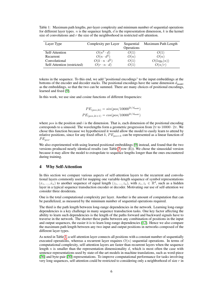
Table 1: Maximum path lengths, per-layer complexity and minimum number of sequential operations
for different layer types. n is the sequence length, d is the representation dimension, k is the kernel
size of convolutions and r the size of the neighborhood in restricted self-attention.
Layer Type
Complexity per Layer
Self-Attention
Recurrent
Convolutional
Self-Attention (restricted)
O(n2 · d)
O(n · d2)
O(k · n · d2)
O(r · n · d)
Sequential Maximum Path Length
Operations
O(1)
O(n)
O(1)
O(1)
O(1)
O(n)
O(logk(n))
O(n/r)
tokens in the sequence. To this end, we add "positional encodings" to the input embeddings at the
bottoms of the encoder and decoder stacks. The positional encodings have the same dimension dmodel
as the embeddings, so that the two can be summed. There are many choices of positional encodings,
learned and fixed [9].
In this work, we use sine and cosine functions of different frequencies:
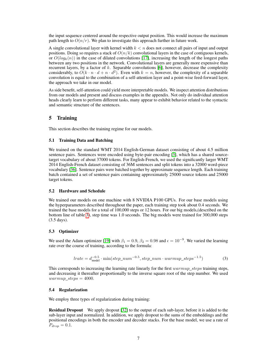
P E(pos,2i) = sin(pos/100002i/dmodel)
P E(pos,2i+1) = cos(pos/100002i/dmodel)
where pos is the position and i is the dimension. That is, each dimension of the positional encoding
corresponds to a sinusoid. The wavelengths form a geometric progression from 2π to 10000 · 2π. We
chose this function because we hypothesized it would allow the model to easily learn to attend by
relative positions, since for any fixed offset k, P Epos+k can be represented as a linear function of
P Epos.
We also experimented with using learned positional embeddings [9] instead, and found that the two
versions produced nearly identical results (see Table 3 row (E)). We chose the sinusoidal version
because it may allow the model to extrapolate to sequence lengths longer than the ones encountered
during training.
4 Why Self-Attention
In this section we compare various aspects of self-attention layers to the recurrent and convolu-
tional layers commonly used for mapping one variable-length sequence of symbol representations
(x1, ..., xn) to another sequence of equal length (z1, ..., zn), with xi, zi ∈ Rd, such as a hidden
layer in a typical sequence transduction encoder or decoder. Motivating our use of self-attention we
consider three desiderata.
One is the total computational complexity per layer. Another is the amount of computation that can
be parallelized, as measured by the minimum number of sequential operations required.
The third is the path length between long-range dependencies in the network. Learning long-range
dependencies is a key challenge in many sequence transduction tasks. One key factor affecting the
ability to learn such dependencies is the length of the paths forward and backward signals have to
traverse in the network. The shorter these paths between any combination of positions in the input
and output sequences, the easier it is to learn long-range dependencies [12]. Hence we also compare
the maximum path length between any two input and output positions in networks composed of the
different layer types.
As noted in Table 1, a self-attention layer connects all positions with a constant number of sequentially
executed operations, whereas a recurrent layer requires O(n) sequential operations. In terms of
computational complexity, self-attention layers are faster than recurrent layers when the sequence
length n is smaller than the representation dimensionality d, which is most often the case with
sentence representations used by state-of-the-art models in machine translations, such as word-piece
[36] and byte-pair [30] representations. To improve computational performance for tasks involving
very long sequences, self-attention could be restricted to considering only a neighborhood of size r in
6
�
the input sequence centered around the respective output position. This would increase the maximum
path length to O(n/r). We plan to investigate this approach further in future work.
A single convolutional layer with kernel width k < n does not connect all pairs of input and output
positions. Doing so requires a stack of O(n/k) convolutional layers in the case of contiguous kernels,
or O(logk(n)) in the case of dilated convolutions [17], increasing the length of the longest paths
between any two positions in the network. Convolutional layers are generally more expensive than
recurrent layers, by a factor of k. Separable convolutions [6], however, decrease the complexity
considerably, to O(k · n · d + n · d2). Even with k = n, however, the complexity of a separable
convolution is equal to the combination of a self-attention layer and a point-wise feed-forward layer,
the approach we take in our model.
As side benefit, self-attention could yield more interpretable models. We inspect attention distributions
from our models and present and discuss examples in the appendix. Not only do individual attention
heads clearly learn to perform different tasks, many appear to exhibit behavior related to the syntactic
and semantic structure of the sentences.
5 Training
This section describes the training regime for our models.
5.1 Training Data and Batching
We trained on the standard WMT 2014 English-German dataset consisting of about 4.5 million
sentence pairs. Sentences were encoded using byte-pair encoding [3], which has a shared source-
target vocabulary of about 37000 tokens. For English-French, we used the significantly larger WMT
2014 English-French dataset consisting of 36M sentences and split tokens into a 32000 word-piece
vocabulary [36]. Sentence pairs were batched together by approximate sequence length. Each training
batch contained a set of sentence pairs containing approximately 25000 source tokens and 25000
target tokens.
5.2 Hardware and Schedule
We trained our models on one machine with 8 NVIDIA P100 GPUs. For our base models using
the hyperparameters described throughout the paper, each training step took about 0.4 seconds. We
trained the base models for a total of 100,000 steps or 12 hours. For our big models,(described on the
bottom line of table 3), step time was 1.0 seconds. The big models were trained for 300,000 steps
(3.5 days).
5.3 Optimizer
We used the Adam optimizer [19] with β1 = 0.9, β2 = 0.98 and � = 10−9. We varied the learning
rate over the course of training, according to the formula:
lrate = d−0.5
model · min(step_num−0.5, step_num · warmup_steps−1.5)
(3)
This corresponds to increasing the learning rate linearly for the first warmup_steps training steps,
and decreasing it thereafter proportionally to the inverse square root of the step number. We used
warmup_steps = 4000.
5.4 Regularization
We employ three types of regularization during training:
Residual Dropout We apply dropout [32] to the output of each sub-layer, before it is added to the
sub-layer input and normalized. In addition, we apply dropout to the sums of the embeddings and the
positional encodings in both the encoder and decoder stacks. For the base model, we use a rate of
Pdrop = 0.1.
7
�
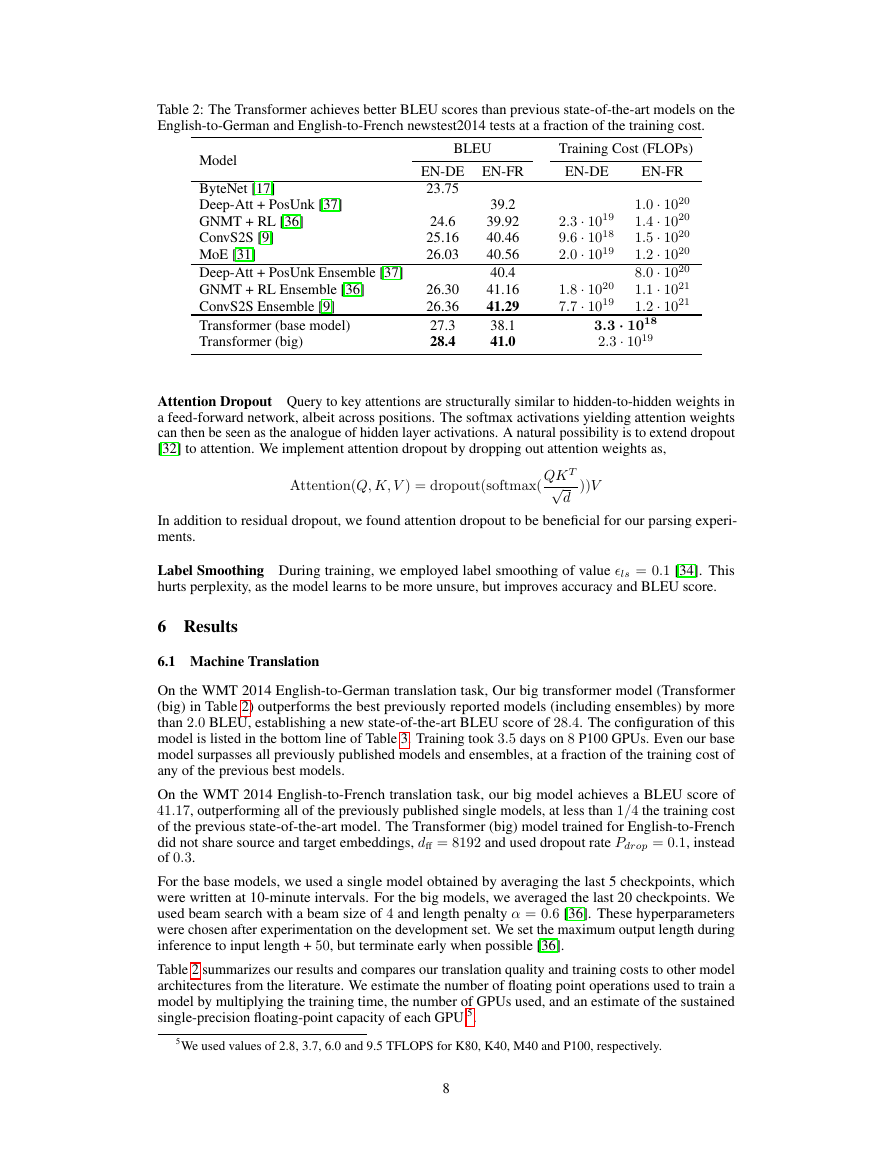
Table 2: The Transformer achieves better BLEU scores than previous state-of-the-art models on the
English-to-German and English-to-French newstest2014 tests at a fraction of the training cost.
Model
ByteNet [17]
Deep-Att + PosUnk [37]
GNMT + RL [36]
ConvS2S [9]
MoE [31]
Deep-Att + PosUnk Ensemble [37]
GNMT + RL Ensemble [36]
ConvS2S Ensemble [9]
Transformer (base model)
Transformer (big)
BLEU
EN-DE EN-FR
23.75
24.6
25.16
26.03
26.30
26.36
27.3
28.4
39.2
39.92
40.46
40.56
40.4
41.16
41.29
38.1
41.0
EN-FR
1.0 · 1020
1.4 · 1020
1.5 · 1020
1.2 · 1020
8.0 · 1020
1.1 · 1021
1.2 · 1021
2.3 · 1019
9.6 · 1018
2.0 · 1019
1.8 · 1020
7.7 · 1019
Training Cost (FLOPs)
EN-DE
3.3 · 1018
2.3 · 1019
Attention Dropout Query to key attentions are structurally similar to hidden-to-hidden weights in
a feed-forward network, albeit across positions. The softmax activations yielding attention weights
can then be seen as the analogue of hidden layer activations. A natural possibility is to extend dropout
[32] to attention. We implement attention dropout by dropping out attention weights as,
Attention(Q, K, V ) = dropout(softmax(
QK T√
d
))V
In addition to residual dropout, we found attention dropout to be beneficial for our parsing experi-
ments.
Label Smoothing During training, we employed label smoothing of value �ls = 0.1 [34]. This
hurts perplexity, as the model learns to be more unsure, but improves accuracy and BLEU score.
6 Results
6.1 Machine Translation
On the WMT 2014 English-to-German translation task, Our big transformer model (Transformer
(big) in Table 2) outperforms the best previously reported models (including ensembles) by more
than 2.0 BLEU, establishing a new state-of-the-art BLEU score of 28.4. The configuration of this
model is listed in the bottom line of Table 3. Training took 3.5 days on 8 P100 GPUs. Even our base
model surpasses all previously published models and ensembles, at a fraction of the training cost of
any of the previous best models.
On the WMT 2014 English-to-French translation task, our big model achieves a BLEU score of
41.17, outperforming all of the previously published single models, at less than 1/4 the training cost
of the previous state-of-the-art model. The Transformer (big) model trained for English-to-French
did not share source and target embeddings, dff = 8192 and used dropout rate Pdrop = 0.1, instead
of 0.3.
For the base models, we used a single model obtained by averaging the last 5 checkpoints, which
were written at 10-minute intervals. For the big models, we averaged the last 20 checkpoints. We
used beam search with a beam size of 4 and length penalty α = 0.6 [36]. These hyperparameters
were chosen after experimentation on the development set. We set the maximum output length during
inference to input length + 50, but terminate early when possible [36].
Table 2 summarizes our results and compares our translation quality and training costs to other model
architectures from the literature. We estimate the number of floating point operations used to train a
model by multiplying the training time, the number of GPUs used, and an estimate of the sustained
single-precision floating-point capacity of each GPU 5.
5We used values of 2.8, 3.7, 6.0 and 9.5 TFLOPS for K80, K40, M40 and P100, respectively.
8
�



 2023年江西萍乡中考道德与法治真题及答案.doc
 2012年重庆南川中考生物真题及答案.doc
 2013年江西师范大学地理学综合及文艺理论基础考研真题.doc
 2020年四川甘孜小升初语文真题及答案I卷.doc
 2020年注册岩土工程师专业基础考试真题及答案.doc
 2023-2024学年福建省厦门市九年级上学期数学月考试题及答案.doc
 2021-2022学年辽宁省沈阳市大东区九年级上学期语文期末试题及答案.doc
 2022-2023学年北京东城区初三第一学期物理期末试卷及答案.doc
 2018上半年江西教师资格初中地理学科知识与教学能力真题及答案.doc
 2012年河北国家公务员申论考试真题及答案-省级.doc
 2020-2021学年江苏省扬州市江都区邵樊片九年级上学期数学第一次质量检测试题及答案.doc
 2022下半年黑龙江教师资格证中学综合素质真题及答案.doc