6
1
0
2
g
u
A
3
1
]
L
M
.
t
a
t
s
[
2
v
8
0
9
5
0
.
6
0
6
1
:
v
i
X
r
a
Tutorial on Variational Autoencoders
CARL DOERSCH
Carnegie Mellon / UC Berkeley
August 16, 2016
Abstract
In just three years, Variational Autoencoders (VAEs) have emerged
as one of the most popular approaches to unsupervised learning of
complicated distributions. VAEs are appealing because they are built
on top of standard function approximators (neural networks), and
can be trained with stochastic gradient descent. VAEs have already
shown promise in generating many kinds of complicated data, in-
cluding handwritten digits [1, 2], faces [1, 3, 4], house numbers [5, 6],
CIFAR images [6], physical models of scenes [4], segmentation [7], and
predicting the future from static images [8]. This tutorial introduces the
intuitions behind VAEs, explains the mathematics behind them, and
describes some empirical behavior. No prior knowledge of variational
Bayesian methods is assumed.
Keywords: variational autoencoders, unsupervised learning, structured
prediction, neural networks
1
Introduction
“Generative modeling” is a broad area of machine learning which deals with
models of distributions P(X), defined over datapoints X in some potentially
high-dimensional space X . For instance, images are a popular kind of data
for which we might create generative models. Each “datapoint” (image) has
thousands or millions of dimensions (pixels), and the generative model’s job
is to somehow capture the dependencies between pixels, e.g., that nearby
pixels have similar color, and are organized into objects. Exactly what it
means to “capture” these dependencies depends on exactly what we want
to do with the model. One straightforward kind of generative model simply
allows us to compute P(X) numerically. In the case of images, X values
1
�
which look like real images should get high probability, whereas images
that look like random noise should get low probability. However, models
like this are not necessarily useful: knowing that one image is unlikely does
not help us synthesize one that is likely.
Instead, one often cares about producing more examples that are like
those already in a database, but not exactly the same. We could start with a
database of raw images and synthesize new, unseen images. We might take
in a database of 3D models of something like plants and produce more of
them to fill a forest in a video game. We could take handwritten text and try
to produce more handwritten text. Tools like this might actually be useful
for graphic designers. We can formalize this setup by saying that we get
examples X distributed according to some unknown distribution Pgt(X),
and our goal is to learn a model P which we can sample from, such that P is
as similar as possible to Pgt.
Training this type of model has been a long-standing problem in the ma-
chine learning community, and classically, most approaches have had one of
three serious drawbacks. First, they might require strong assumptions about
the structure in the data. Second, they might make severe approximations,
leading to suboptimal models. Or third, they might rely on computation-
ally expensive inference procedures like Markov Chain Monte Carlo. More
recently, some works have made tremendous progress in training neural
networks as powerful function approximators through backpropagation [9].
These advances have given rise to promising frameworks which can use
backpropagation-based function approximators to build generative models.
One of the most popular such frameworks is the Variational Autoen-
coder [1, 3], the subject of this tutorial. The assumptions of this model are
weak, and training is fast via backpropagation. VAEs do make an approxi-
mation, but the error introduced by this approximation is arguably small
given high-capacity models. These characteristics have contributed to a
quick rise in their popularity.
This tutorial is intended to be an informal introduction to VAEs, and not
a formal scientific paper about them. It is aimed at people who might have
uses for generative models, but might not have a strong background in the
variatonal Bayesian methods and “minimum description length” coding
models on which VAEs are based. This tutorial began its life as a presentation
for computer vision reading groups at UC Berkeley and Carnegie Mellon,
and hence has a bias toward a vision audience. Suggestions for improvement
are appreciated.
2
�
1.1 Preliminaries: Latent Variable Models
When training a generative model, the more complicated the dependencies
between the dimensions, the more difficult the models are to train. Take,
for example, the problem of generating images of handwritten characters.
Say for simplicity that we only care about modeling the digits 0-9. If the left
half of the character contains the left half of a 5, then the right half cannot
contain the left half of a 0, or the character will very clearly not look like any
real digit. Intuitively, it helps if the model first decides which character to
generate before it assigns a value to any specific pixel. This kind of decision
is formally called a latent variable. That is, before our model draws anything,
it first randomly samples a digit value z from the set [0, ..., 9], and then makes
sure all the strokes match that character. z is called ‘latent’ because given
just a character produced by the model, we don’t necessarily know which
settings of the latent variables generated the character. We would need to
infer it using something like computer vision.
Before we can say that our model is representative of our dataset, we
need to make sure that for every datapoint X in the dataset, there is one (or
many) settings of the latent variables which causes the model to generate
something very similar to X. Formally, say we have a vector of latent
variables z in a high-dimensional space Z which we can easily sample
according to some probability density function (PDF) P(z) defined over Z.
Then, say we have a family of deterministic functions f (z; θ), parameterized
by a vector θ in some space Θ, where f : Z × Θ → X . f is deterministic, but
if z is random and θ is fixed, then f (z; θ) is a random variable in the space
X . We wish to optimize θ such that we can sample z from P(z) and, with
high probability, f (z; θ) will be like the X’s in our dataset.
To make this notion precise mathematically, we are aiming maximize the
probability of each X in the training set under the entire generative process,
according to:
P(X|z; θ)P(z)dz.
P(X) =
(1)
Here, f (z; θ) has been replaced by a distribution P(X|z; θ), which allows us
to make the dependence of X on z explicit by using the law of total probabil-
ity. The intuition behind this framework—called “maximum likelihood”—
is that if the model is likely to produce training set samples, then it is
also likely to produce similar samples, and unlikely to produce dissimilar
ones. In VAEs, the choice of this output distribution is often Gaussian, i.e.,
P(X|z; θ) = N (X| f (z; θ), σ2 ∗ I). That is, it has mean f (z; θ) and covariance
equal to the identity matrix I times some scalar σ (which is a hyperparam-
eter). This replacement is necessary to formalize the intuition that some z
3
�
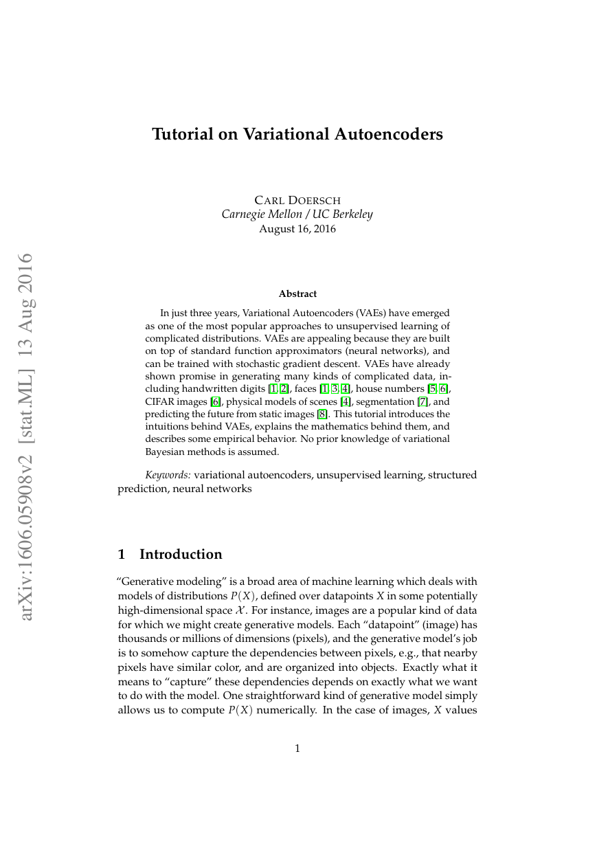
Figure 1: The standard VAE model represented as a graphical model. Note
the conspicuous lack of any structure or even an “encoder” pathway: it is
possible to sample from the model without any input. Here, the rectangle is
“plate notation” meaning that we can sample from z and X N times while
the model parameters θ remain fixed.
needs to result in samples that are merely like X. In general, and particularly
early in training, our model will not produce outputs that are identical to
any particular X. By having a Gaussian distribution, we can use gradient
descent (or any other optimization technique) to increase P(X) by making
f (z; θ) approach X for some z, i.e., gradually making the training data more
likely under the generative model. This wouldn’t be possible if P(X|z) was
a Dirac delta function, as it would be if we used X = f (z; θ) deterministi-
cally! Note that the output distribution is not required to be Gaussian: for
instance, if X is binary, then P(X|z) might be a Bernoulli parameterized by
f (z; θ). The important property is simply that P(X|z) can be computed, and
is continuous in θ. From here onward, we will omit θ from f (z; θ) to avoid
clutter.
2 Variational Autoencoders
The mathematical basis of VAEs actually has relatively little to do with
classical autoencoders, e.g. sparse autoencoders [10, 11] or denoising au-
toencoders [12, 13]. VAEs approximately maximize Equation 1, according
to the model shown in Figure 1. They are called “autoencoders” only be-
cause the final training objective that derives from this setup does have
an encoder and a decoder, and resembles a traditional autoencoder. Unlike
sparse autoencoders, there are generally no tuning parameters analogous to
the sparsity penalties. And unlike sparse and denoising autoencoders, we
4
�
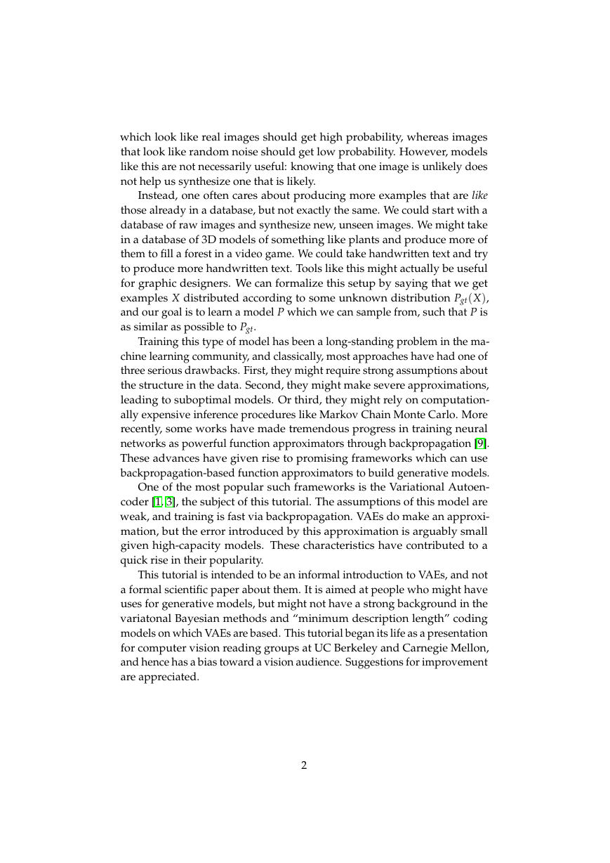
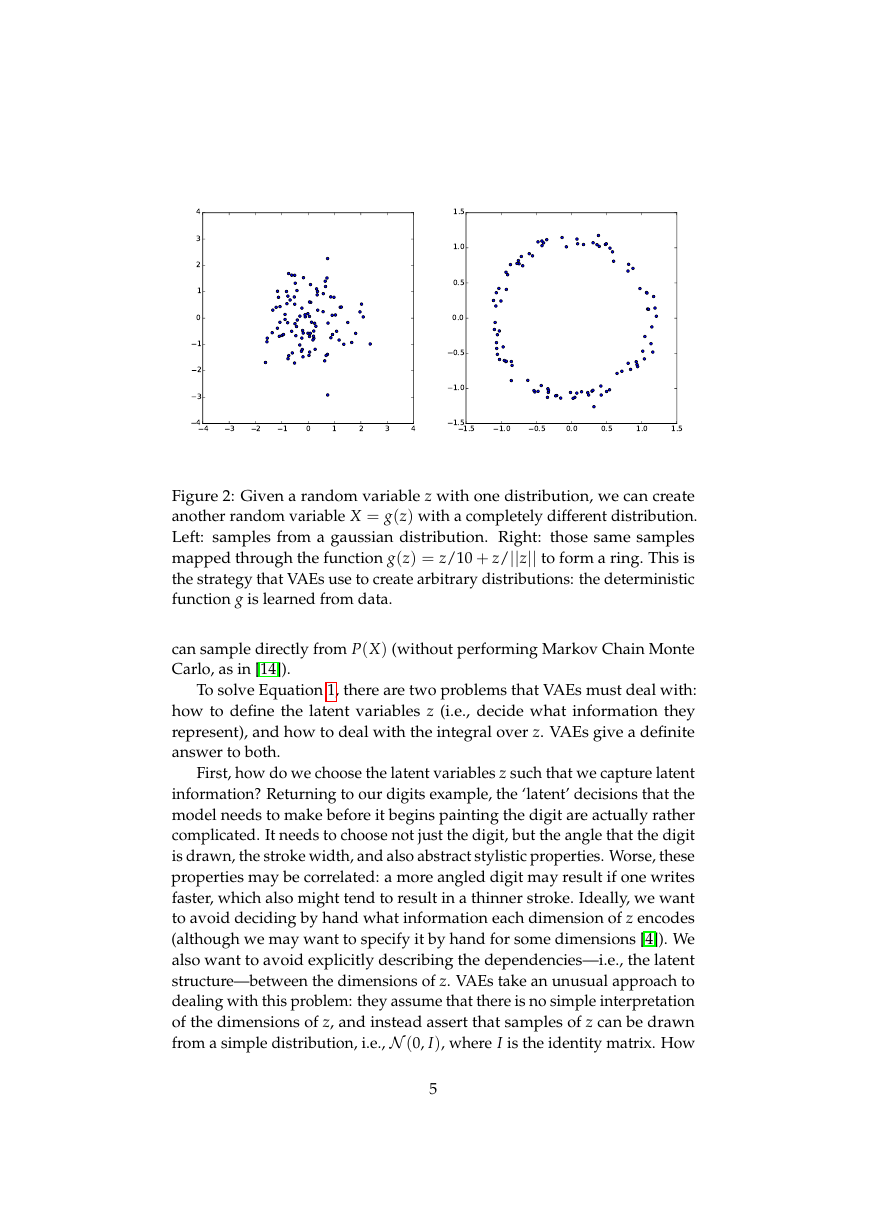
Figure 2: Given a random variable z with one distribution, we can create
another random variable X = g(z) with a completely different distribution.
Left: samples from a gaussian distribution. Right: those same samples
mapped through the function g(z) = z/10 + z/||z|| to form a ring. This is
the strategy that VAEs use to create arbitrary distributions: the deterministic
function g is learned from data.
can sample directly from P(X) (without performing Markov Chain Monte
Carlo, as in [14]).
To solve Equation 1, there are two problems that VAEs must deal with:
how to define the latent variables z (i.e., decide what information they
represent), and how to deal with the integral over z. VAEs give a definite
answer to both.
First, how do we choose the latent variables z such that we capture latent
information? Returning to our digits example, the ‘latent’ decisions that the
model needs to make before it begins painting the digit are actually rather
complicated. It needs to choose not just the digit, but the angle that the digit
is drawn, the stroke width, and also abstract stylistic properties. Worse, these
properties may be correlated: a more angled digit may result if one writes
faster, which also might tend to result in a thinner stroke. Ideally, we want
to avoid deciding by hand what information each dimension of z encodes
(although we may want to specify it by hand for some dimensions [4]). We
also want to avoid explicitly describing the dependencies—i.e., the latent
structure—between the dimensions of z. VAEs take an unusual approach to
dealing with this problem: they assume that there is no simple interpretation
of the dimensions of z, and instead assert that samples of z can be drawn
from a simple distribution, i.e., N (0, I), where I is the identity matrix. How
5
4321012344321012341.51.00.50.00.51.01.51.51.00.50.00.51.01.5�
(a)
(b)
(c)
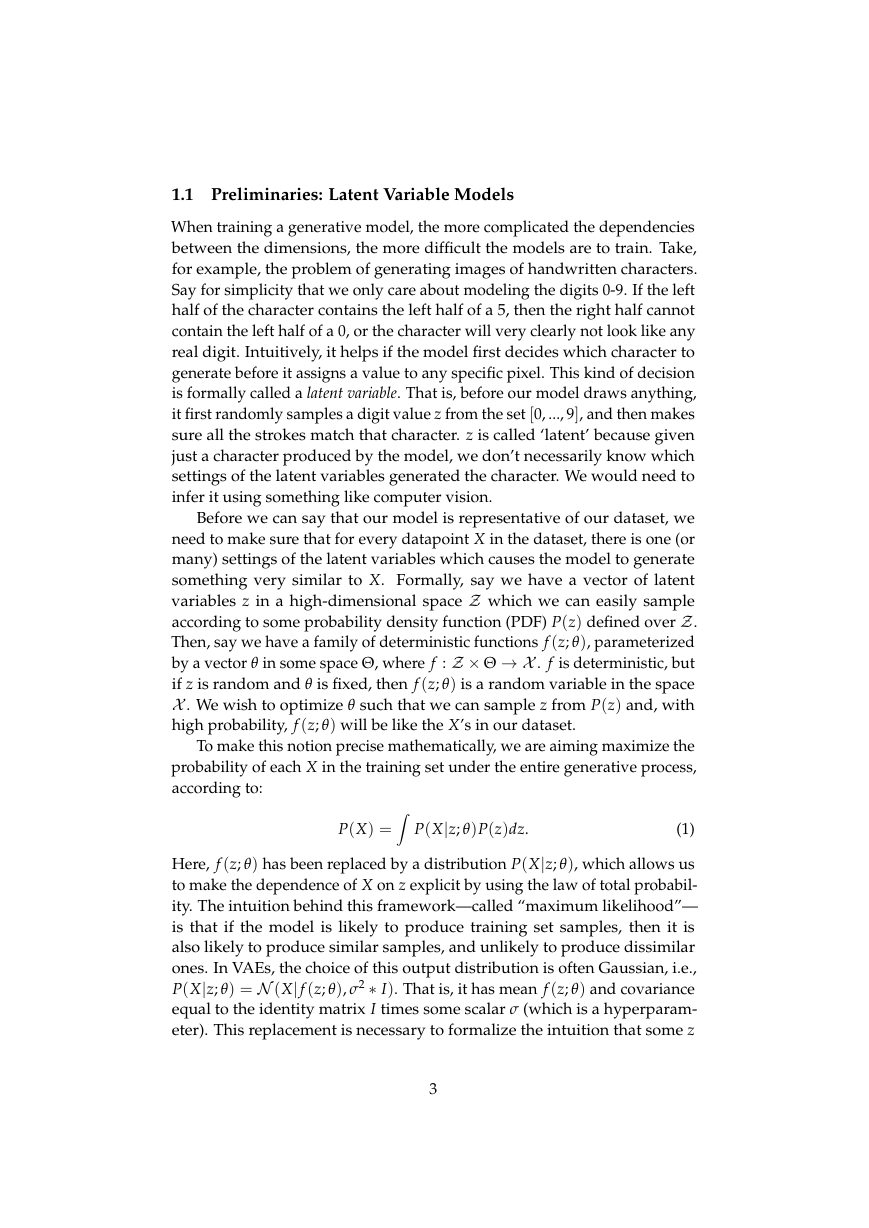
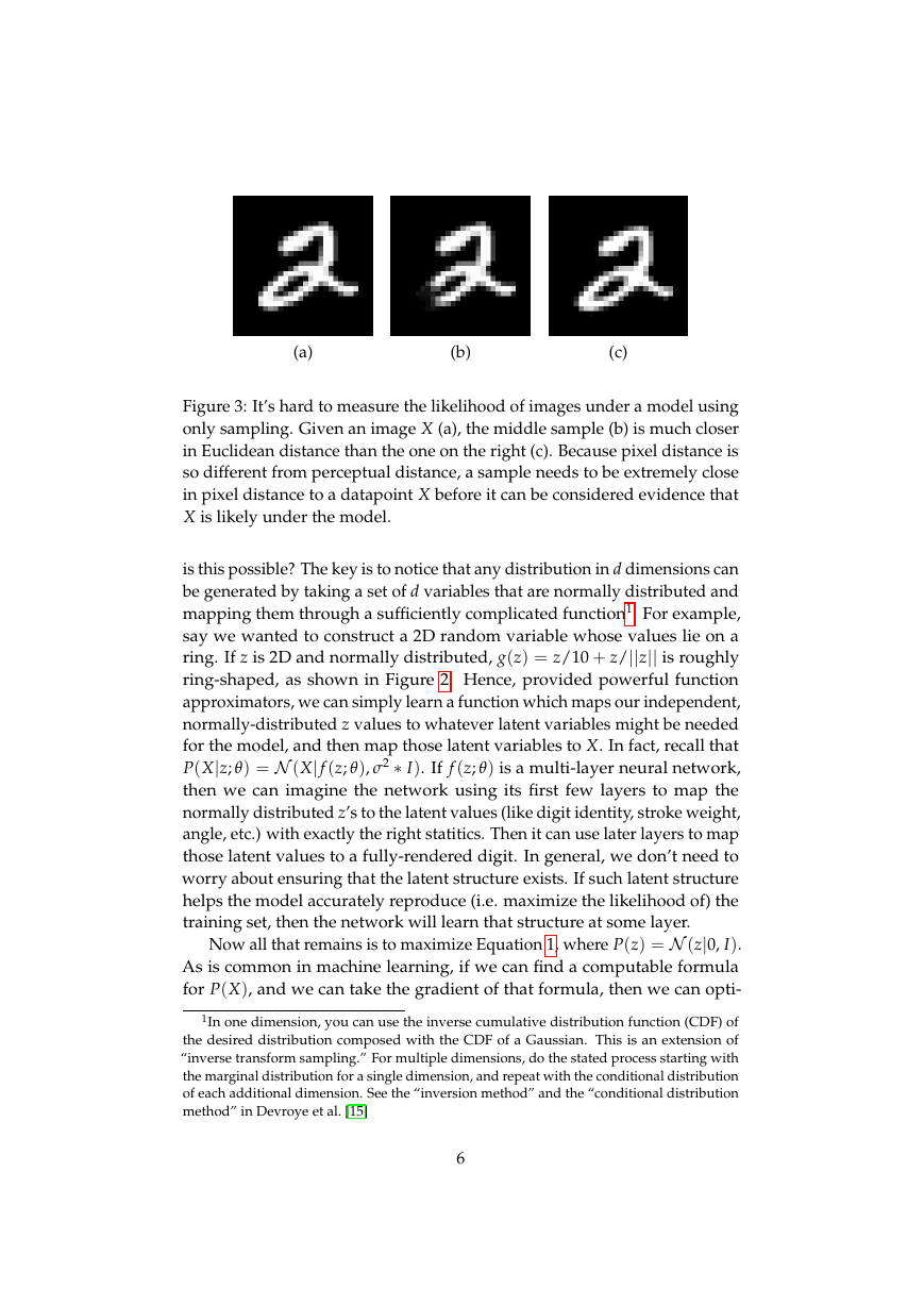
Figure 3: It’s hard to measure the likelihood of images under a model using
only sampling. Given an image X (a), the middle sample (b) is much closer
in Euclidean distance than the one on the right (c). Because pixel distance is
so different from perceptual distance, a sample needs to be extremely close
in pixel distance to a datapoint X before it can be considered evidence that
X is likely under the model.
is this possible? The key is to notice that any distribution in d dimensions can
be generated by taking a set of d variables that are normally distributed and
mapping them through a sufficiently complicated function1. For example,
say we wanted to construct a 2D random variable whose values lie on a
ring. If z is 2D and normally distributed, g(z) = z/10 + z/||z|| is roughly
ring-shaped, as shown in Figure 2. Hence, provided powerful function
approximators, we can simply learn a function which maps our independent,
normally-distributed z values to whatever latent variables might be needed
for the model, and then map those latent variables to X. In fact, recall that
P(X|z; θ) = N (X| f (z; θ), σ2 ∗ I). If f (z; θ) is a multi-layer neural network,
then we can imagine the network using its first few layers to map the
normally distributed z’s to the latent values (like digit identity, stroke weight,
angle, etc.) with exactly the right statitics. Then it can use later layers to map
those latent values to a fully-rendered digit. In general, we don’t need to
worry about ensuring that the latent structure exists. If such latent structure
helps the model accurately reproduce (i.e. maximize the likelihood of) the
training set, then the network will learn that structure at some layer.
Now all that remains is to maximize Equation 1, where P(z) = N (z|0, I).
As is common in machine learning, if we can find a computable formula
for P(X), and we can take the gradient of that formula, then we can opti-
1In one dimension, you can use the inverse cumulative distribution function (CDF) of
the desired distribution composed with the CDF of a Gaussian. This is an extension of
“inverse transform sampling.” For multiple dimensions, do the stated process starting with
the marginal distribution for a single dimension, and repeat with the conditional distribution
of each additional dimension. See the “inversion method” and the “conditional distribution
method” in Devroye et al. [15]
6
�
n
mize the model using stochastic gradient ascent. It is actually conceptually
straightforward to compute P(X) approximately: we first sample a large
number of z values {z1, ..., zn}, and compute P(X) ≈ 1
∑i P(X|zi). The prob-
lem here is that in high dimensional spaces, n might need to be extremely
large before we have an accurate estimate of P(X). To see why, consider
our example of handwritten digits. Say that our digit datapoints are stored
in pixel space, in 28x28 images as shown in Figure 3. Since P(X|z) is an
isotropic Gaussian, the negative log probability of X is proportional squared
Euclidean distance between f (z) and X. Say that Figure 3(a) is the target
(X) for which we are trying to find P(X). A model which produces the
image shown in Figure 3(b) is probably a bad model, since this digit is not
much like a 2. Hence, we should set the σ hyperparameter of our Gaussian
distribution such that this kind of erroroneous digit does not contribute to
P(X). On the other hand, a model which produces Figure 3(c) (identical to
X but shifted down and to the right by half a pixel) might be a good model.
We would hope that this sample would contribute to P(X). Unfortunately,
however, we can’t have it both ways: the squared distance between X and
Figure 3(c) is .2693 (assuming pixels range between 0 and 1), but between
X and Figure 3(b) it is just .0387. The lesson here is that in order to reject
samples like Figure 3(b), we need to set σ very small, such that the model
needs to generate something significantly more like X than Figure 3(c)! Even
if our model is an accurate generator of digits, we would likely need to
sample many thousands of digits before we produce a 2 that is sufficiently
similar to the one in Figure 3(a). We might solve this problem by using
a better similarity metric, but in practice these are difficult to engineer in
complex domains like vision, and they’re difficult to train without labels
that indicate which datapoints are similar to each other. Instead, VAEs alter
the sampling procedure to make it faster, without changing the similarity
metric.
2.1 Setting up the objective
Is there a shortcut we can take when using sampling to compute Equation 1?
In practice, for most z, P(X|z) will be nearly zero, and hence contribute
almost nothing to our estimate of P(X). The key idea behind the variational
autoencoder is to attempt to sample values of z that are likely to have
produced X, and compute P(X) just from those. This means that we need a
new function Q(z|X) which can take a value of X and give us a distribution
over z values that are likely to produce X. Hopefully the space of z values
that are likely under Q will be much smaller than the space of all z’s that are
likely under the prior P(z). This lets us, for example, compute Ez∼QP(X|z)
relatively easily. However, if z is sampled from an arbitrary distribution
7
�
with PDF Q(z), which is not N (0, I), then how does that help us optimize
P(X)? The first thing we need to do is relate Ez∼QP(X|z) and P(X). We’ll
see where Q comes from later.
The relationship between Ez∼QP(X|z) and P(X) is one of the corner-
stones of variational Bayesian methods. We begin with the definition of
Kullback-Leibler divergence (KL divergence or D) between P(z|X) and
Q(z), for some arbitrary Q (which may or may not depend on X):
D [Q(z)P(z|X)] = Ez∼Q [log Q(z) − log P(z|X)] .
(2)
We can get both P(X) and P(X|z) into this equation by applying Bayes rule
to P(z|X):
D [Q(z)P(z|X)] = Ez∼Q [log Q(z) − log P(X|z) − log P(z)] + log P(X).
(3)
Here, log P(X) comes out of the expectation because it does not depend on
z. Negating both sides, rearranging, and contracting part of Ez∼Q into a
KL-divergence terms yields:
log P(X) − D [Q(z)P(z|X)] = Ez∼Q [log P(X|z)] − D [Q(z)P(z)] .
(4)
Note that X is fixed, and Q can be any distribution, not just a distribution
which does a good job mapping X to the z’s that can produce X. Since we’re
interested in inferring P(X), it makes sense to construct a Q which does
depend on X, and in particular, one which makes D [Q(z)|P(z|X)] small:
log P(X) − D [Q(z|X)P(z|X)] = Ez∼Q [log P(X|z)] − D [Q(z|X)P(z)] .
(5)
This equation serves is the core of the variational autoencoder, and it’s worth
spending some time thinking about what it says2. In two sentences, the left
hand side has the quantity we want to maximize: log P(X) (plus an error
term, which makes Q produce z’s that can reproduce a given X; this term
will become small if Q is high-capacity). The right hand side is something
we can optimize via stochastic gradient descent given the right choice of
Q (although it may not be obvious yet how). Note that the framework—in
particular, the right hand side of Equation 5—has suddenly taken a form
which looks like an autoencoder, since Q is “encoding” X into z, and P is
“decoding” it to reconstruct X. We’ll explore this connection in more detail
later.
2 Historically, this math (particularly Equation 5) was known long before VAEs. For
example, Helmholtz Machines [16] (see Equation 5) use nearly identical mathematics, with
one crucial difference. The integral in our expectations is replaced with a sum in Dayan et
al. [16], because Helmholtz Machines assume a discrete distribution for the latent variables.
This choice prevents the transformations that make gradient descent tractable in VAEs.
8
�


 2023年江西萍乡中考道德与法治真题及答案.doc
 2012年重庆南川中考生物真题及答案.doc
 2013年江西师范大学地理学综合及文艺理论基础考研真题.doc
 2020年四川甘孜小升初语文真题及答案I卷.doc
 2020年注册岩土工程师专业基础考试真题及答案.doc
 2023-2024学年福建省厦门市九年级上学期数学月考试题及答案.doc
 2021-2022学年辽宁省沈阳市大东区九年级上学期语文期末试题及答案.doc
 2022-2023学年北京东城区初三第一学期物理期末试卷及答案.doc
 2018上半年江西教师资格初中地理学科知识与教学能力真题及答案.doc
 2012年河北国家公务员申论考试真题及答案-省级.doc
 2020-2021学年江苏省扬州市江都区邵樊片九年级上学期数学第一次质量检测试题及答案.doc
 2022下半年黑龙江教师资格证中学综合素质真题及答案.doc