0
2
0
2
r
a
M
2
1
]
G
L
.
s
c
[
1
v
9
8
6
5
0
.
3
0
0
2
:
v
i
X
r
a
Hyper-Parameter Optimization: A Review of Algorithms and Applications
Hyper-Parameter Optimization: A Review of Algorithms
and Applications
Tong Yu
Department of AI and HPC
Inspur Electronic Information Industry Co., Ltd
1036 Langchao Rd, Jinan, Shandong, China
Hong Zhu
Department of AI and HPC
Inspur (Beijing) Electronic Information Industry Co., Ltd
2F, Block C, 2 Xinxi Rd., Shangdi, Haidian Dist, Beijing, China
yutong01@inspur.com
zhuhongbj@inspur.com
Editor:
Abstract
Since deep neural networks were developed, they have made huge contributions to peoples
everyday lives. Machine learning provides more rational advice than humans are capable
of in almost every aspect of daily life. However, despite this achievement, the design and
training of neural networks are still challenging and unpredictable procedures that have
been alleged to be alchemy. To lower the technical thresholds for common users, automated
hyper-parameter optimization (HPO) has become a popular topic in both academic and
industrial areas. This paper provides a review of the most essential topics on HPO. The
first section introduces the key hyper-parameters related to model training and structure,
and discusses their importance and methods to define the value range. Then, the research
focuses on major optimization algorithms and their applicability, covering their efficiency
and accuracy especially for deep learning networks. This study next reviews major services
and tool-kits for HPO, comparing their support for state-of-the-art searching algorithms,
feasibility with major deep-learning frameworks, and extensibility for new modules designed
by users. The paper concludes with problems that exist when HPO is applied to deep
learning, a comparison between optimization algorithms, and prominent approaches for
model evaluation with limited computational resources.
Keywords: Hyper-parameter, auto-tuning, deep neural network
1. Introduction
In the past several years, neural network techniques have become ubiquitous and influ-
ential in both research and commercial applications. In the past 10 years, neural networks
have shown impressive results in image classification (Szegedy et al., 2016; He et al., 2016),
objective detection (Girshick, 2015; Redmon et al., 2016), natural language understand-
ing (Hochreiter and Schmidhuber, 1997; Vaswani et al., 2017), and industrial control sys-
tems (Abbeel, 2016; Hammond, 2017).However, neural networks are efficient in applications
but inefficient when obtaining a model. It is thought to be a brute force method because a
network is initialized with a random status and trained to an accurate model with an ex-
tremely large dataset. Moreover, researchers must dedicate their efforts to carefully coping
1
�
Yu and Zhu
with model design, algorithm design, and corresponding hyper-parameter selection, which
means that the application of neural networks comes at a great price. Based on experience is
generally the most widely used method, which means a practicable set of hyper-parameters
requires researchers to have experience in training neural networks. However, the credibil-
ity of empirical values is weakened because of the lack of logical reasoning. In addition,
experiences generally provide workable instead of optimal hyper-parameter sets.
The no free lunch theorem suggests that the computational cost for any optimiza-
tion problem is the same for all problems and no solution offers a shortcut (Wolpert and
Macready, 1997; Igel, 2014).A feasible alternative for computational resources is the pre-
liminary knowledge of experts, which is efficient in selecting influential parameters and
narrowing down the search space. To save the rare resource of experts experience, auto-
mated machine learning (AutoML) has been proposed as a burgeoning technology to design
and train neural networks automatically, at the cost of computational resources (Feurer
et al., 2015; Katz et al., 2016; Bello et al., 2017; Zoph and Le, 2016; Jin et al., 2018).Hyper-
parameter optimization (HPO) is an important component of AutoML in searching for
optimum hyper-parameters for neural network structures and the model training process.
Hyper-parameter refers to parameters that cannot be updated during the training of
machine learning. They can be involved in building the structure of the model, such as
the number of hidden layers and the activation function, or in determining the efficiency
and accuracy of model training, such as the learning rate (LR) of stochastic gradient de-
scent (SGD), batch size, and optimizer (hyp).The history of HPO dates back to the early
1990s (Ripley, 1993; King et al., 1995),and the method is widely applied for neural net-
works with the increasing use of machine learning. HPO can be viewed as the final step of
model design and the first step of training a neural network. Considering the influence of
hyper-parameters on training accuracy and speed, they must carefully be configured with
experience before the training process begins (Rodriguez, 2018). The process of HPO auto-
matically optimizes the hyper-parameters of a machine learning model to remove humans
from the loop of a machine learning system. As a trade of human efforts, HPO demands
a large amount of computational resources, especially when several hyper-parameters are
optimized together. The questions of how to utilize computational resources and design an
efficient search space have resulted in various studies on HPO on algorithms and toolkits.
Conceptually, HPOs purposes are threefold (Feurer and Hutter, 2019): to reduce the costly
menial work of artificial intelligence (AI) experts and lower the threshold of research and
development; to improve the accuracy and efficiency of neural network training (Melis et al.,
2017); and to make the choice of hyper-parameter set more convincing and the training re-
sults more reproducible (Bergstra et al., 2013).
In recent years, HPO has become increasingly necessary because of two rising trends
in the development of deep learning models. The first trend is the upscaling of neural
networks for enhanced accuracy (Tan and Le, 2019).Empirical studies have indicated that
in most cases, more complex machine learning models with deeper and wider layers work
better than do those with simple structures (He et al., 2016; Zagoruyko and Komodakis,
2016; Huang et al., 2019).The second trend is to design a tricky lightweight model to pro-
vide satisfying accuracy with fewer weights and parameters (Ma et al., 2018; Sandler et al.,
2018; Tan et al., 2019). In this case, it is more difficult to adapt empirical values because
of the stricter choices of hyper-parameters. Hyper-parameter tuning plays an essential role
2
�
Hyper-Parameter Optimization: A Review of Algorithms and Applications
in both cases: a model with a complex structure indicates more hyper-parameters to tune,
and a model with a carefully designed structure implies that every hyper-parameter must
be tuned to a strict range to reproduce the accuracy. For a widely used model, tuning its
hyper-parameters by hand is possible because the ability to tune by hand depends on ex-
perience and researchers can always borrow knowledge from previous works. This is similar
for models at a small scale. However, for a larger model or newly published models, the
wide range of hyper-parameter choices requires a great deal of menial work by researchers,
as well as much time and computational resources for trial and error.
In addition to research, the industrial application of deep learning is a crucial practice in
automobiles, manufacturing, and digital assistants. However, even for trained professional
researchers, it is still no easy task to explore and implement a favorable model to solve
specific problems. Users with less experience have substantial needs for suggested hyper-
parameters and ready-to-use HPO tools. Motivated by both academic needs and practical
application, automated hyper-parameter tuning services (Golovin et al., 2017; Amazon,
2018)and toolkits (Liaw et al., 2018; Microsoft, 2018)provide a solution to the limitation of
manual deep learning designs.
This study is motivated by the prosperous demand for design and training deep learning
network in industry and research. The difficulty in selecting proper parameters for different
tasks makes it necessary to summarize existing algorithms and tools. The objective of this
research is to conduct a survey on feasible algorithms for HPO, make a comparison on lead-
ing tools for HPO tasks, and propose challenges on HPO tasks on deep learning networks.
Thus, this remainder of this paper is structured as follows. Section 2 begins with a dis-
cussion of key hyper-parameters for building and training neural networks, including their
influence on models, potential search spaces, and empirical values or schedules based on pre-
vious experience. Section 3 focuses on widely used algorithms in hyper-parameter searching,
and these approaches are categorized into searching algorithms and trial schedulers. This
section also evaluates the efficiency and applicability of these algorithms for different ma-
chine learning models. Section 4 provides an overview of mainstream HPO toolkits and
services, compares their pros and cons, and presents some practical and implementation de-
tails. Section 5 more comprehensively compares existing HPO methods and highlights the
efficient methods of model evaluation, and finally, Section 6 provides the studys conclusions.
The contribution of this study is summarized as follows:
- Hyper-parameters are systematically categorized into structure-related and training-
related. The discussion of their importance and empirical strategies are helpful to
determine which hyper-parameters are involved in HPO.
- HPO algorithms are analyzed and compared in detail, according to their accuracy,
efficiency and scope of application. The analysis on previous studies is not only
committed to include state-of-the-art algorithms, but also to clarify limitations on
certain scenarios.
- By comparing HPO toolkits, this study gives insights of the design of close-sourced
libraries and open-sourced services, and clarifies the targeted users for each of them.
3
�
Yu and Zhu
- The potential research direction regarding to existing problems are suggested on al-
gorithms, applications and techniques.
2. Major Hyper-Parameters and Search Space
Considering the computational resources required, hyper-parameters with greater im-
portance receive preferential treatment in the process of HPO. Hyper-parameters with a
stronger effect on weights during training are more influential for neural network train-
ing (Ng, 2017). It is difficult to quantitatively determine which of the hyper-parameters
are the most significant for final accuracy. In general, there are more studies on those with
higher importance, and their importance has been decided by previous experience.
Hyper-parameters can be categorized into two groups: those used for training and those
used for model design. A proper choice of hyper-parameters related to model training al-
lows neural networks to learn faster and achieve enhanced performance. Currently, the most
adopted optimizer for training a deep neural network is stochastic gradient descent (Rob-
bins and Monro, 1951) with momentum (Qian, 1999) as well as its variants such as Ada-
Grad (Duchi et al., 2011), RMSprop (Hinton et al., 2012a), and Adam (Kingma and Ba,
2014). In addition to the choice of optimizer, corresponding hyper-parameters (e.g., mo-
mentum) are critical for certain networks. During the training process, batch size and LR
draw the most attention because they determine the speed of convergence, the tuning of
which should always be ensured. Hyper-parameters for model design are more related to
the structure of neural networks, the most typical example being the number of hidden
layers and width of layers. These hyper-parameters usually measure the models learning
capacity, which is determined by the complexity of function (Agrawal, 2018).
This section provides an in-depth discussion on hyper-parameters of great importance
for model structures and training, as well as introduce their effect in models and provide
suggested values or schedules.
2.1 Learning Rate
LR is a positive scalar that determines the length of step during SGD (Goodfellow
et al., 2016).
In most cases, the LR must be manually adjusted during model training,
and this adjustment is often necessary for enhanced accuracy (Bengio, 2012).An alternative
choice of fixed LR is a varied LR over the training process. This method is referred to as
the LR schedule or LR decay (Goodfellow et al., 2016). Adaptive LR can be adjusted in
response to the performance or structure of the model, and it is supported by a learning
algorithm (Smith, 2017; Brownlee, 2019).
Constant LR, as the simplest schedule, is often set as the default by deep learning
frameworks (e.g., Keras).
It is an important but tricky task to determine a good value
for LR. With a proper constant LR, the network is able to be trained to a passable but
unsatisfactory accuracy because the initial value could always be overlarge, especially in
the final few steps. A small improvement based on the constant value is to set an initial
rate as 0.1, for example, adjusting to 0.01 when the accuracy is saturated, and to 0.001 if
necessary (nachiket tanksale, 2018).
Linear LR decay is a common choice for researchers who wish to set a schedule.
It
changes gradually during the training process based on time or step. The basic mathematical
4
�
Hyper-Parameter Optimization: A Review of Algorithms and Applications
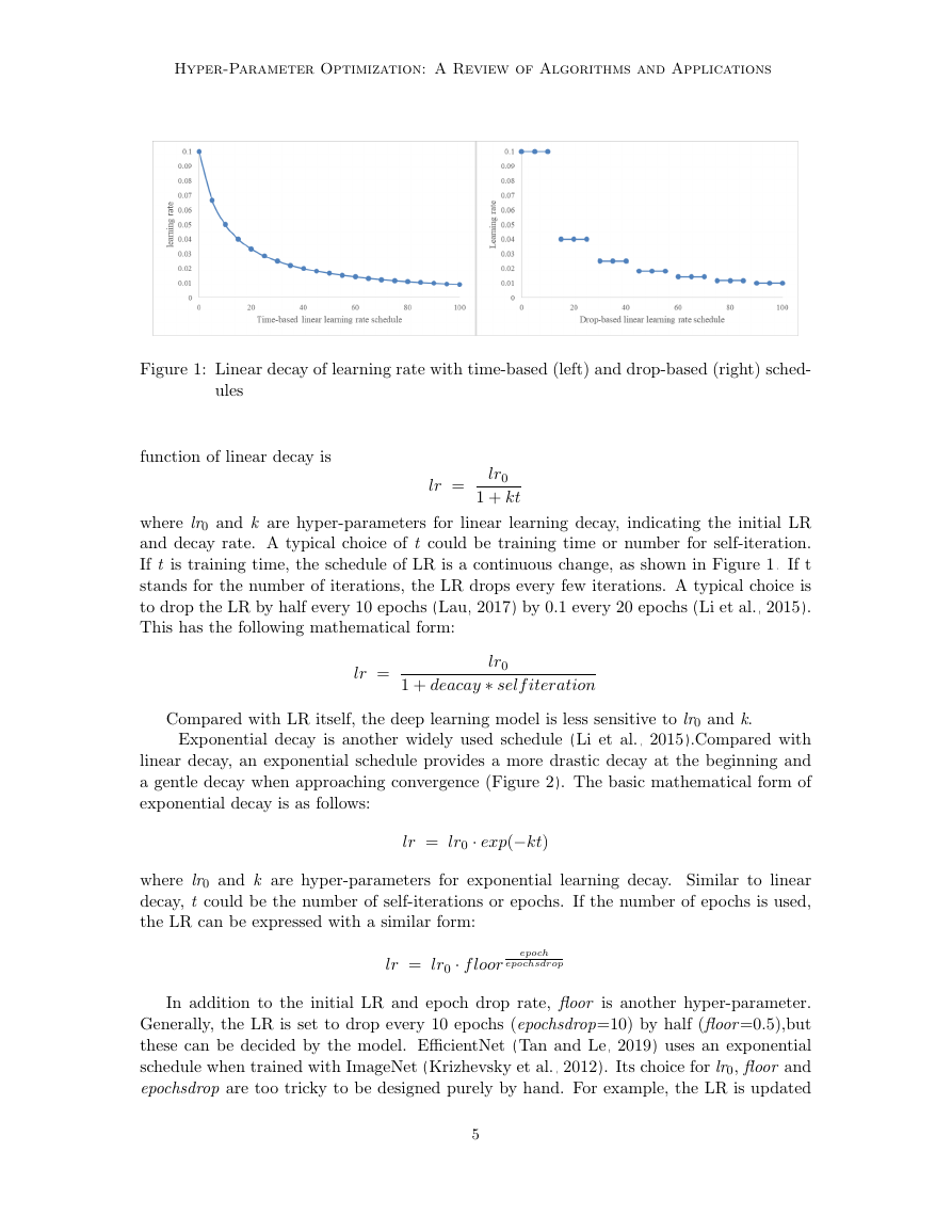
Figure 1: Linear decay of learning rate with time-based (left) and drop-based (right) sched-
ules
function of linear decay is
lr =
lr0
1 + kt
where lr0 and k are hyper-parameters for linear learning decay, indicating the initial LR
and decay rate. A typical choice of t could be training time or number for self-iteration.
If t is training time, the schedule of LR is a continuous change, as shown in Figure 1. If t
stands for the number of iterations, the LR drops every few iterations. A typical choice is
to drop the LR by half every 10 epochs (Lau, 2017) by 0.1 every 20 epochs (Li et al., 2015).
This has the following mathematical form:
lr =
lr0
1 + deacay ∗ self iteration
Compared with LR itself, the deep learning model is less sensitive to lr0 and k.
Exponential decay is another widely used schedule (Li et al., 2015).Compared with
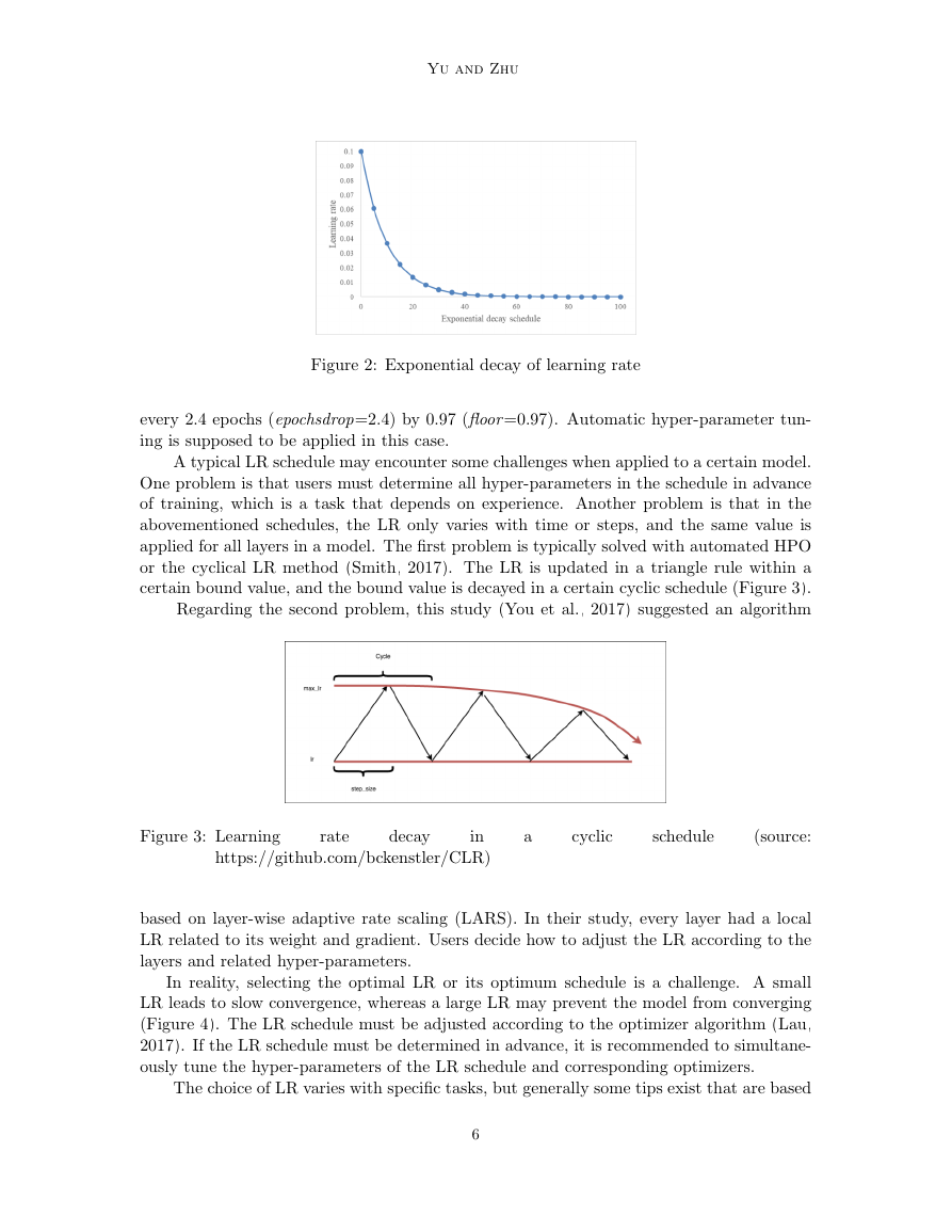
linear decay, an exponential schedule provides a more drastic decay at the beginning and
a gentle decay when approaching convergence (Figure 2). The basic mathematical form of
exponential decay is as follows:
lr = lr0 · exp(−kt)
where lr0 and k are hyper-parameters for exponential learning decay. Similar to linear
decay, t could be the number of self-iterations or epochs. If the number of epochs is used,
the LR can be expressed with a similar form:
lr = lr0 · f loor
epoch
epochsdrop
In addition to the initial LR and epoch drop rate, floor is another hyper-parameter.
Generally, the LR is set to drop every 10 epochs (epochsdrop=10) by half (floor =0.5),but
these can be decided by the model. EfficientNet (Tan and Le, 2019) uses an exponential
schedule when trained with ImageNet (Krizhevsky et al., 2012). Its choice for lr0, floor and
epochsdrop are too tricky to be designed purely by hand. For example, the LR is updated
5
�
Yu and Zhu
Figure 2: Exponential decay of learning rate
every 2.4 epochs (epochsdrop=2.4) by 0.97 (floor =0.97). Automatic hyper-parameter tun-
ing is supposed to be applied in this case.
A typical LR schedule may encounter some challenges when applied to a certain model.
One problem is that users must determine all hyper-parameters in the schedule in advance
of training, which is a task that depends on experience. Another problem is that in the
abovementioned schedules, the LR only varies with time or steps, and the same value is
applied for all layers in a model. The first problem is typically solved with automated HPO
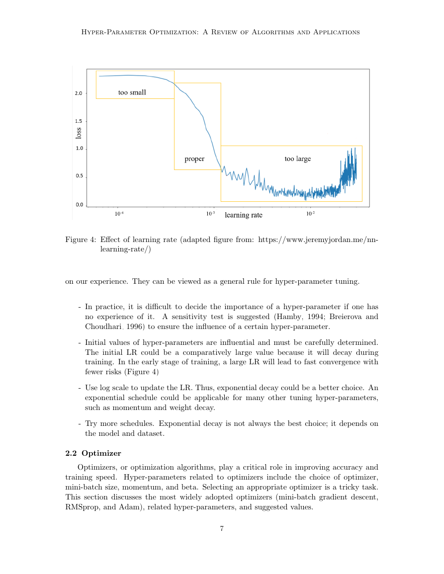
or the cyclical LR method (Smith, 2017). The LR is updated in a triangle rule within a
certain bound value, and the bound value is decayed in a certain cyclic schedule (Figure 3).
Regarding the second problem, this study (You et al., 2017) suggested an algorithm
Figure 3: Learning
rate
in
https://github.com/bckenstler/CLR)
decay
a
cyclic
schedule
(source:
based on layer-wise adaptive rate scaling (LARS). In their study, every layer had a local
LR related to its weight and gradient. Users decide how to adjust the LR according to the
layers and related hyper-parameters.
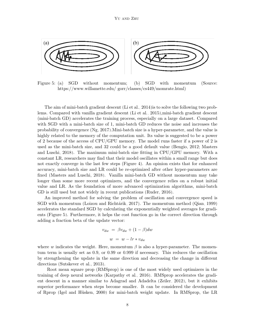
In reality, selecting the optimal LR or its optimum schedule is a challenge. A small
LR leads to slow convergence, whereas a large LR may prevent the model from converging
(Figure 4). The LR schedule must be adjusted according to the optimizer algorithm (Lau,
2017). If the LR schedule must be determined in advance, it is recommended to simultane-
ously tune the hyper-parameters of the LR schedule and corresponding optimizers.
The choice of LR varies with specific tasks, but generally some tips exist that are based
6
�
Hyper-Parameter Optimization: A Review of Algorithms and Applications
Figure 4: Effect of learning rate (adapted figure from: https://www.jeremyjordan.me/nn-
learning-rate/)
on our experience. They can be viewed as a general rule for hyper-parameter tuning.
- In practice, it is difficult to decide the importance of a hyper-parameter if one has
no experience of it. A sensitivity test is suggested (Hamby, 1994; Breierova and
Choudhari, 1996) to ensure the influence of a certain hyper-parameter.
- Initial values of hyper-parameters are influential and must be carefully determined.
The initial LR could be a comparatively large value because it will decay during
training. In the early stage of training, a large LR will lead to fast convergence with
fewer risks (Figure 4)
- Use log scale to update the LR. Thus, exponential decay could be a better choice. An
exponential schedule could be applicable for many other tuning hyper-parameters,
such as momentum and weight decay.
- Try more schedules. Exponential decay is not always the best choice; it depends on
the model and dataset.
2.2 Optimizer
Optimizers, or optimization algorithms, play a critical role in improving accuracy and
training speed. Hyper-parameters related to optimizers include the choice of optimizer,
mini-batch size, momentum, and beta. Selecting an appropriate optimizer is a tricky task.
This section discusses the most widely adopted optimizers (mini-batch gradient descent,
RMSprop, and Adam), related hyper-parameters, and suggested values.
7
�
Yu and Zhu
Figure 5: (a)
SGD without momentum;
(b)
SGD with momentum (Source:
https://www.willamette.edu/ gorr/classes/cs449/momrate.html)
The aim of mini-batch gradient descent (Li et al., 2014)is to solve the following two prob-
lems. Compared with vanilla gradient descent (Li et al., 2015),mini-batch gradient descent
(mini-batch GD) accelerates the training process, especially on a large dataset. Compared
with SGD with a mini-batch size of 1, mini-batch GD reduces the noise and increases the
probability of convergence (Ng, 2017).Mini-batch size is a hyper-parameter, and the value is
highly related to the memory of the computation unit. Its value is suggested to be a power
of 2 because of the access of CPU/GPU memory. The model runs faster if a power of 2 is
used as the mini-batch size, and 32 could be a good default value (Bengio, 2012; Masters
and Luschi, 2018). The maximum mini-batch size fitting in CPU/GPU memory. With a
constant LR, researchers may find that their model oscillates within a small range but does
not exactly converge in the last few steps (Figure 4). An opinion exists that for enhanced
accuracy, mini-batch size and LR could be re-optimized after other hyper-parameters are
fixed (Masters and Luschi, 2018). Vanilla mini-batch GD without momentum may take
longer than some more recent optimizers, and the convergence relies on a robust initial
value and LR. As the foundation of more advanced optimization algorithms, mini-batch
GD is still used but not widely in recent publications (Ruder, 2016).
An improved method for solving the problem of oscillation and convergence speed is
SGD with momentum (Loizou and Richt´arik, 2017). The momentum method (Qian, 1999)
accelerates the standard SGD by calculating the exponentially weighted averages for gradi-
ents (Figure 5). Furthermore, it helps the cost function go in the correct direction through
adding a fraction beta of the update vector:
vdw = βvdw + (1 − β)dw
w = w − lr ∗ vdw
where w indicates the weight. Here, momentum β is also a hyper-parameter. The momen-
tum term is usually set as 0.9, or 0.99 or 0.999 if necessary. This reduces the oscillation
by strengthening the update in the same direction and decreasing the change in different
directions (Sutskever et al., 2013).
Root mean square prop (RMSprop) is one of the most widely used optimizers in the
training of deep neural networks (Karpathy et al., 2016). RMSprop accelerates the gradi-
ent descent in a manner similar to Adagrad and Adadelta (Zeiler, 2012), but it exhibits
superior performance when steps become smaller. It can be considered the development
In RMSprop, the LR
of Rprop (Igel and H¨usken, 2000) for mini-batch weight update.
8
�


 2023年江西萍乡中考道德与法治真题及答案.doc
 2012年重庆南川中考生物真题及答案.doc
 2013年江西师范大学地理学综合及文艺理论基础考研真题.doc
 2020年四川甘孜小升初语文真题及答案I卷.doc
 2020年注册岩土工程师专业基础考试真题及答案.doc
 2023-2024学年福建省厦门市九年级上学期数学月考试题及答案.doc
 2021-2022学年辽宁省沈阳市大东区九年级上学期语文期末试题及答案.doc
 2022-2023学年北京东城区初三第一学期物理期末试卷及答案.doc
 2018上半年江西教师资格初中地理学科知识与教学能力真题及答案.doc
 2012年河北国家公务员申论考试真题及答案-省级.doc
 2020-2021学年江苏省扬州市江都区邵樊片九年级上学期数学第一次质量检测试题及答案.doc
 2022下半年黑龙江教师资格证中学综合素质真题及答案.doc