cs231n_完整版笔记.pdf-资料库

professionall-9630743-4744300845234085292.pdf-第1页.png

第1页 / 共191页

professionall-9630743-4744300845234085292.pdf-第2页.png

第2页 / 共191页

professionall-9630743-4744300845234085292.pdf-第3页.png

第3页 / 共191页

professionall-9630743-4744300845234085292.pdf-第4页.png

第4页 / 共191页

professionall-9630743-4744300845234085292.pdf-第5页.png

第5页 / 共191页

professionall-9630743-4744300845234085292.pdf-第6页.png

第6页 / 共191页

professionall-9630743-4744300845234085292.pdf-第7页.png

第7页 / 共191页

professionall-9630743-4744300845234085292.pdf-第8页.png

第8页 / 共191页

Convolutional Neural Networks for Visual Recognition Feifei Li CS231n, Stanford Open Course

Edited by fengfu-chris, email: fengfu0527@gmail.com Copyright: Stanford Vision Group Contents Part I: Neural Networks 1.1 - Image Classification: Data-driven Approach, k-Nearest Neighbor, train/val/test splits ------- 3 1.2 - Linear classification: Support Vector Machine, Softmax ------------------------------------------ 19 1.3 - Optimization: Stochastic Gradient Descent ---------------------------------------------------------- 37 1.4 - Backpropagation, Intuitions ---------------------------------------------------------------------------- 51 1.5 - Neural Networks Part 1: Setting up the Architecture ----------------------------------------------- 60 1.6 - Neural Networks Part 2: Setting up the Data and the Loss ---------------------------------------- 73 1.7 - Neural Networks Part 3: Learning and Evaluation -------------------------------------------------- 89 1.8 - Putting it together: Minimal Neural Network Case Study ---------------------------------------- 109 Part II: Convolutional Neural Networks 2.1 - Convolutional Neural Networks: Architectures, Convolution & Pooling Layers ------------- 123 2.2 - Understanding and Visualizing Convolutional Neural Networks ------------------------------- 146 2.3 - Transfer Learning and Fine-tuning Convolutional Neural Networks --------------------------- 152 2.4 - ConvNet Tips and Tricks: squeezing out the last few percent ----------------------------------- 155 Part X: Preparation x.1 - Python Numpy Tutorial ------------------------------------------------------------------------------- 156 x.2 - IPython Tutorial ---------------------------------------------------------------------------------------- 182 x.3 - Terminal ------------------------------------------------------------------------------------------------- 186

CS231n Convolutional Neural Networks for Visual Recognition These notes accompany the Stanford CS class CS231n: Convolutional Neural Networks for Visual Recognition. Feel free to ping @karpathy if you spot any mistakes or issues, or submit a pull request to our git repo. We encourage the use of the hypothes.is extension to annote comments and discuss these notes inline. Assignments Assignment #1: Image Classification, kNN, SVM, Softmax Assignment #2: Neural Networks, ConvNets I Assignment #3: ConvNets II, Transfer Learning, Visualization Module 0: Preparation Python / Numpy Tutorial IPython Notebook Tutorial Terminal.com Tutorial Module 1: Neural Networks Image Classification: Data-driven Approach, k-Nearest Neighbor, train/val/test splits L1/L2 distances, hyperparameter search, cross-validation Linear classification: Support Vector Machine, Softmax parameteric approach, bias trick, hinge loss, cross-entropy loss, L2 regularization, web demo Optimization: Stochastic Gradient Descent optimization landscapes, local search, learning rate, analytic/numerical gradient Backpropagation, Intuitions chain rule interpretation, real-valued circuits, patterns in gradient flow Neural Networks Part 1: Setting up the Architecture 1

model of a biological neuron, activation functions, neural net architecture, representational power Neural Networks Part 2: Setting up the Data and the Loss preprocessing, weight initialization, regularization, dropout, loss functions in the wild Neural Networks Part 3: Learning and Evaluation gradient checks, sanity checks, babysitting the learning process, momentum (+nesterov), second-order methods, Adagrad/RMSprop, hyperparameter optimization, model ensembles Putting it together: Minimal Neural Network Case Study minimal 2D toy data example Module 2: Convolutional Neural Networks Convolutional Neural Networks: Architectures, Convolution / Pooling Layers layers, spatial arrangement, layer patterns, layer sizing patterns, AlexNet/ZFNet/VGGNet case studies, computational considerations Understanding and Visualizing Convolutional Neural Networks tSNE embeddings, deconvnets, data gradients, fooling ConvNets, human comparisons Transfer Learning and Fine-tuning Convolutional Neural Networks ConvNet Tips and Tricks: squeezing out the last few percent multi-scale, model ensembles, data augmentations Module 3: ConvNets in the wild Other Visual Recognition Tasks: Localization, Detection, Segmentation ConvNets in Practice: Distributed Training, GPU bottlenecks, Libraries cs231n cs231n karpathy@cs.stanford.edu 2

CS231n Convolutional Neural Networks for Visual Recognition This is an introductory lecture designed to introduce people from outside of Computer Vision to the Image Classification problem, and the data-driven approach. The Table of Contents: Intro to Image Classification, data-driven approach, pipeline Nearest Neighbor Classifier k-Nearest Neighbor Validation sets, Cross-validation, hyperparameter tuning Pros/Cons of Nearest Neighbor Summary Summary: Applying kNN in practice Further Reading Image Classification Motivation. In this section we will introduce the Image Classification problem, which is the task of assigning an input image one label from a fixed set of categories. This is one of the core problems in Computer Vision that, despite its simplicity, has a large variety of practical applications. Moreover, as we will see later in the course, many other seemingly distinct Computer Vision tasks (such as object detection, segmentation) can be reduced to image classification. 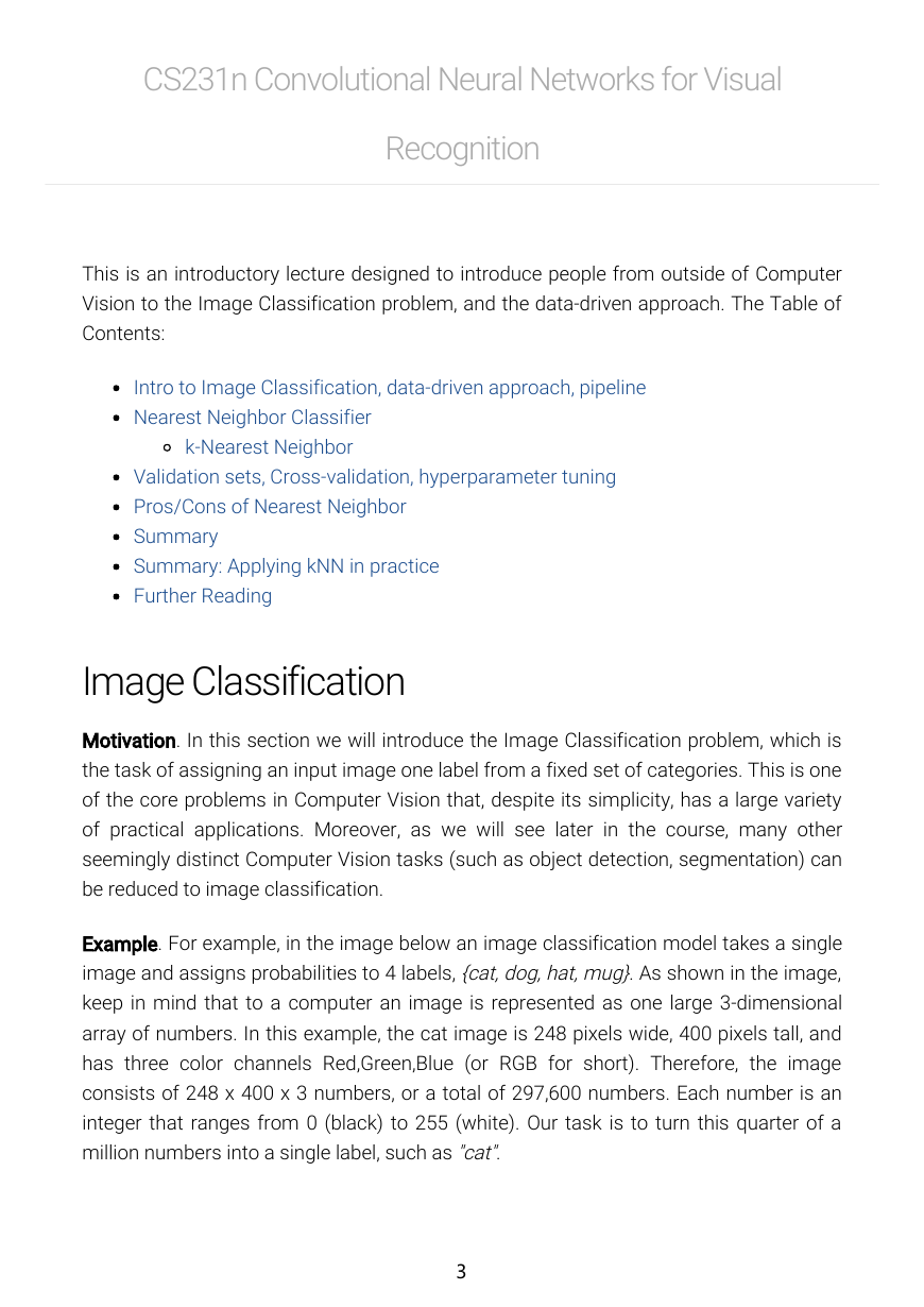Example. For example, in the image below an image classification model takes a single image and assigns probabilities to 4 labels, {cat, dog, hat, mug}. As shown in the image, keep in mind that to a computer an image is represented as one large 3-dimensional array of numbers. In this example, the cat image is 248 pixels wide, 400 pixels tall, and has three color channels Red,Green,Blue (or RGB for short). Therefore, the image consists of 248 x 400 x 3 numbers, or a total of 297,600 numbers. Each number is an integer that ranges from 0 (black) to 255 (white). Our task is to turn this quarter of a million numbers into a single label, such as "cat". 3

The task in Image Classification is to predict a single label (or a distribution over labels as shown here to indicate our confidence) for a given image. Images are 3-dimensional arrays of integers from 0 to 255, of size Width x Height x 3. The 3 represents the three color channels Red, Green, Blue. Challenges. Since this task of recognizing a visual concept (e.g. cat) is relatively trivial for a human to perform, it is worth considering the challenges involved from the perspective of a Computer Vision algorithm. 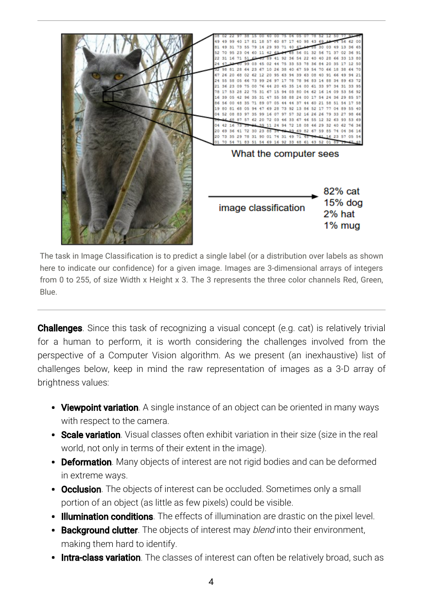As we present (an inexhaustive) list of challenges below, keep in mind the raw representation of images as a 3-D array of brightness values: Viewpoint variation. A single instance of an object can be oriented in many ways with respect to the camera. Scale variation. Visual classes often exhibit variation in their size (size in the real world, not only in terms of their extent in the image). Deformation. Many objects of interest are not rigid bodies and can be deformed in extreme ways. Occlusion. The objects of interest can be occluded. Sometimes only a small portion of an object (as little as few pixels) could be visible. Illumination conditions. The effects of illumination are drastic on the pixel level. Background clutter. The objects of interest may blend into their environment, making them hard to identify. Intra-class variation. The classes of interest can often be relatively broad, such as 4

chair. There are many different types of these objects, each with their own appearance. A good image classification model must be invariant to the cross product of all these variations, while simultaneously retaining sensitivity to the inter-class variations. Data-driven approach. How might we go about writing an algorithm that can classify images into distinct categories? Unlike writing an algorithm for, for example, sorting a list of numbers, it is not obvious how one might write an algorithm for identifying cats in images. 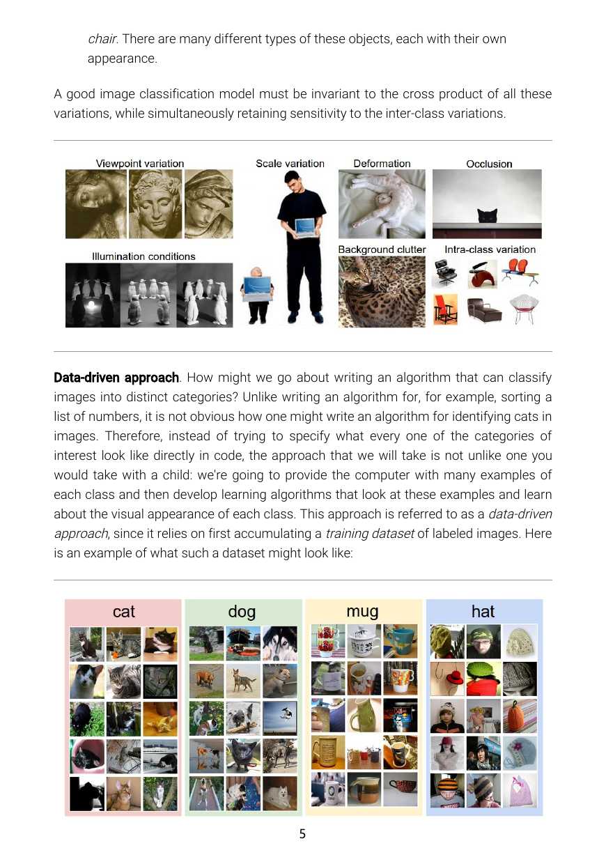Therefore, instead of trying to specify what every one of the categories of interest look like directly in code, the approach that we will take is not unlike one you would take with a child: we're going to provide the computer with many examples of each class and then develop learning algorithms that look at these examples and learn about the visual appearance of each class. This approach is referred to as a data-driven approach, since it relies on first accumulating a training dataset of labeled images. Here is an example of what such a dataset might look like: 5

An example training set for four visual categories. In practice we may have thousands of categories and hundreds of thousands of images for each category. The image classification pipeline. We've seen that the task in Image Classification is to take an array of pixels that represents a single image and assign a label to it. Our complete pipeline can be formalized as follows: Input: Our input consists of a set of N images, each labeled with one of K different classes. We refer to this data as the training set. Learning: Our task is to use the training set to learn what every one of the classes looks like. We refer to this step as training a classifier, or learning a model. Evaluation: In the end, we evaluate the quality of the classifier by asking it to predict labels for a new set of images that it has never seen before. We will then compare the true labels of these images to the ones predicted by the classifier. Intuitively, we're hoping that a lot of the predictions match up with the true answers (which we call the ground truth). Nearest Neighbor Classifier As our first approach, we will develop what we call a Nearest Neighbor Classifier. This classifier has nothing to do with Convolutional Neural Networks and it is very rarely used in practice, but it will allow us to get an idea about the basic approach to an image classification problem. Example image classification dataset: CIFAR-10. One popular toy image classification dataset is the CIFAR-10 dataset. This dataset consists of 60,000 tiny images that are 32 pixels high and wide. Each image is labeled with one of 10 classes (for example "airplane, automobile, bird, etc"). These 60,000 images are partitioned into a training set of 50,000 images and a test set of 10,000 images. In the image below you can see 10 random example images from each one of the 10 classes: 6

资料库

cs231n_完整版笔记.pdf

相关推荐

课程资源

热门标签

最新资料