Forecasting: Principles and Practice
Rob J Hyndman and George Athanasopoulos
Monash University, Australia
From: http://otexts.org/fpp2/
Preface
Welcome to our online textbook on forecasting.
This textbook is intended to provide a comprehensive introduction to
forecasting methods and to present enough information about each
method for readers to be able to use them sensibly. We don’t attempt to
give a thorough discussion of the theoretical details behind each method,
although the references at the end of each chapter will fill in many of
those details.
The book is written for three audiences: (1) people finding themselves
doing forecasting in business when they may not have had any formal
training in the area; (2) undergraduate students studying business;
(3) MBA students doing a forecasting elective. We use it ourselves for a
third-year subject for students undertaking a Bachelor of Commerce or a
Bachelor of Business degree at Monash University, Australia.
For most sections, we only assume that readers are familiar with
introductory statistics, and with high-school algebra. There are a couple
of sections that also require knowledge of matrices, but these are
flagged.
At the end of each chapter we provide a list of “further reading”. In
general, these lists comprise suggested textbooks that provide a more
advanced or detailed treatment of the subject. Where there is no suitable
textbook, we suggest journal articles that provide more information.
We use R throughout the book and we intend students to learn how to
forecast with R. R is free and available on almost every operating system.
It is a wonderful tool for all statistical analysis, not just for forecasting. See
the Using R appendix for instructions on installing and using R.
All R examples in the book assume you have loaded the fpp2 package,
available on CRAN, using library(fpp2). This will automatically load
several other packages including forecast and ggplot2, as well as all the
data used in the book. The fpp2 package requires at least version 8.0 of the forecast package and version 2.0.0 of the ggplot2 package.
We will use the ggplot2 package for all graphics. If you want to learn how to modify the graphs, or create your own ggplot2 graphics that are different from
the examples shown in this book, please either read the ggplot2 book (Wickham 2016), or do the ggplot2 course on the DataCamp online learning
platform.
There is also a DataCamp course based on this book which provides an introduction to some of the ideas in Chapters 2, 3, 7 and 8, plus a brief glimpse at
a few of the topics in Chapters 9 and 11.
The book is different from other forecasting textbooks in several ways.
It is free and online, making it accessible to a wide audience.
It uses R, which is free, open-source, and extremely powerful software.
The online version is continuously updated. You don’t have to wait until the next edition for errors to be removed or new methods to be discussed. We
will update the book frequently.
There are dozens of real data examples taken from our own consulting practice. We have worked with hundreds of businesses and organizations
helping them with forecasting issues, and this experience has contributed directly to many of the examples given here, as well as guiding our general
philosophy of forecasting.
We emphasise graphical methods more than most forecasters. We use graphs to explore the data, analyse the validity of the models fitted and
present the forecasting results.
Changes in the second edition
�
The most important change in edition 2 of the book is that we have restricted our focus to time series forecasting. That is, we no longer consider the
problem of cross-sectional prediction. Instead, all forecasting in this book concerns prediction of data at future times using observations collected in the
past.
We have also simplified the chapter on exponential smoothing, and added new chapters on dynamic regression forecasting, hierarchical forecasting and
practical forecasting issues. We have added new material on combining forecasts, handling complicated seasonality patterns, dealing with hourly, daily
and weekly data, forecasting count time series, and we have many new examples. We have also revised all existing chapters to bring them up-to-date
with the latest research, and we have carefully gone through every chapter to improve the explanations where possible, to add newer references, to add
more exercises, and to make the R code simpler.
Helpful readers of the earlier versions of the book let us know of any typos or errors they had found. These were updated immediately online. No doubt we
have introduced some new mistakes, and we will correct them online as soon as they are spotted. Please continue to let us know about such things.
Please note
This second edition is now almost complete, although we still plan to change a few of the examples. The print version should be available on Amazon by
March 2018.
We have used the latest v8.3 of the forecast package in preparing this book. The current CRAN version is 8.2, and a few examples will not work if you
have v8.2. To install v8.3, use
# install.packages("devtools")
devtools::install_github("robjhyndman/forecast")
Happy forecasting!
Rob J Hyndman and George Athanasopoulos
December 2017
Bibliography
Wickham, Hadley. 2016. ggplot2: Elegant Graphics for Data Analysis. 2nd ed. Springer.
Chapter 1 Getting started
Forecasting has fascinated people for thousands of years, sometimes being considered a sign of divine inspiration, and sometimes being seen as a
criminal activity. The Jewish prophet Isaiah wrote in about 700 BC
Tell us what the future holds, so we may know that you are gods.
(Isaiah 41:23)
One hundred years later, in ancient Babylon, forecasters would foretell the future based on the distribution of maggots in a rotten sheep’s liver. By 300 BC,
people wanting forecasts would journey to Delphi in Greece to consult the Oracle, who would provide her predictions while intoxicated by ethylene
vapours. Forecasters had a tougher time under the emperor Constantine, who issued a decree in AD357 forbidding anyone “to consult a soothsayer, a
mathematician, or a forecaster
it became an offence to defraud by charging money for predictions. The punishment was three months’ imprisonment with hard labour!
May curiosity to foretell the future be silenced forever.” A similar ban on forecasting occurred in England in 1736 when
The varying fortunes of forecasters arise because good forecasts can seem almost magical, while bad forecasts may be dangerous. Consider the
following famous predictions about computing.
I think there is a world market for maybe five computers. (Chairman of IBM, 1943)
Computers in the future may weigh no more than 1.5 tons. (Popular Mechanics, 1949)
There is no reason anyone would want a computer in their home. (President, DEC, 1977)
The last of these was made only three years before IBM produced the first personal computer. Not surprisingly, you can no longer buy a DEC computer.
Forecasting is obviously a difficult activity, and businesses that do it well have a big advantage over those whose forecasts fail.
In this book, we will explore the most reliable methods for producing forecasts. The emphasis will be on methods that are replicable and testable, and
have been shown to work.
1.1 What can be forecast?
Forecasting is required in many situations: deciding whether to build another power generation plant in the next five years requires forecasts of future
demand; scheduling staff in a call centre next week requires forecasts of call volumes; stocking an inventory requires forecasts of stock requirements.
Forecasts can be required several years in advance (for the case of capital investments), or only a few minutes beforehand (for telecommunication
routing). Whatever the circumstances or time horizons involved, forecasting is an important aid to effective and efficient planning.
…
�
Some things are easier to forecast than others. The time of the sunrise tomorrow morning can be forecast very precisely. On the other hand, tomorrow’s
lotto numbers cannot be forecast with any accuracy. The predictability of an event or a quantity depends on several factors including:
1. how well we understand the factors that contribute to it;
2. how much data are available;
3. whether the forecasts can affect the thing we are trying to forecast.
For example, forecasts of electricity demand can be highly accurate because all three conditions are usually satisfied. We have a good idea of the
contributing factors: electricity demand is driven largely by temperatures, with smaller effects for calendar variation such as holidays, and economic
conditions. Provided there is a sufficient history of data on electricity demand and weather conditions, and we have the skills to develop a good model
linking electricity demand and the key driver variables, the forecasts can be remarkably accurate.
On the other hand, when forecasting currency exchange rates, only one of the conditions is satisfied: there is plenty of available data. However, we have a
very limited understanding of the factors that affect exchange rates, and forecasts of the exchange rate have a direct effect on the rates themselves. If
there are well-publicized forecasts that the exchange rate will increase, then people will immediately adjust the price they are willing to pay and so the
forecasts are self-fulfilling. In a sense, the exchange rates become their own forecasts. This is an example of the “efficient market hypothesis”.
Consequently, forecasting whether the exchange rate will rise or fall tomorrow is about as predictable as forecasting whether a tossed coin will come down
as a head or a tail. In both situations, you will be correct about 50% of the time, whatever you forecast. In situations like this, forecasters need to be aware
of their own limitations, and not claim more than is possible.
Often in forecasting, a key step is knowing when something can be forecast accurately, and when forecasts will be no better than tossing a coin. Good
forecasts capture the genuine patterns and relationships which exist in the historical data, but do not replicate past events that will not occur again. In this
book, we will learn how to tell the difference between a random fluctuation in the past data that should be ignored, and a genuine pattern that should be
modelled and extrapolated.
Many people wrongly assume that forecasts are not possible in a changing environment. Every environment is changing, and a good forecasting model
captures the way in which things are changing. Forecasts rarely assume that the environment is unchanging. What is normally assumed is that the way in
which the environment is changing will continue into the future. That is, a highly volatile environment will continue to be highly volatile; a business with
fluctuating sales will continue to have fluctuating sales; and an economy that has gone through booms and busts will continue to go through booms and
busts. A forecasting model is intended to capture the way things move, not just where things are. As Abraham Lincoln said, “If we could first know where
we are and whither we are tending, we could better judge what to do and how to do it”.
Forecasting situations vary widely in their time horizons, factors determining actual outcomes, types of data patterns, and many other aspects.
Forecasting methods can be very simple, such as using the most recent observation as a forecast (which is called the “naïve method”), or highly complex,
such as neural nets and econometric systems of simultaneous equations. Sometimes, there will be no data available at all. For example, we may wish to
forecast the sales of a new product in its first year, but there are obviously no data to work with. In situations like this, we use judgmental forecasting,
discussed in Chapter 4. The choice of method depends on what data are available and the predictability of the quantity to be forecast.
1.2 Forecasting, planning and goals
Forecasting is a common statistical task in business, where it helps to inform decisions about the scheduling of production, transportation and personnel,
and provides a guide to long-term strategic planning. However, business forecasting is often done poorly, and is frequently confused with planning and
goals. They are three different things.
Forecasting
is about predicting the future as accurately as possible, given all of the information available, including historical data and knowledge of any future
events that might impact the forecasts.
Goals
are what you would like to have happen. Goals should be linked to forecasts and plans, but this does not always occur. Too often, goals are set
without any plan for how to achieve them, and no forecasts for whether they are realistic.
Planning
is a response to forecasts and goals. Planning involves determining the appropriate actions that are required to make your forecasts match your
goals.
Forecasting should be an integral part of the decision-making activities of management, as it can play an important role in many areas of a company.
Modern organizations require short-term, medium-term and long-term forecasts, depending on the specific application.
Short-term forecasts
are needed for the scheduling of personnel, production and transportation. As part of the scheduling process, forecasts of demand are often also
required.
Medium-term forecasts
are needed to determine future resource requirements, in order to purchase raw materials, hire personnel, or buy machinery and equipment.
Long-term forecasts
are used in strategic planning. Such decisions must take account of market opportunities, environmental factors and internal resources.
�
An organization needs to develop a forecasting system that involves several approaches to predicting uncertain events. Such forecasting systems require
the development of expertise in identifying forecasting problems, applying a range of forecasting methods, selecting appropriate methods for each
problem, and evaluating and refining forecasting methods over time. It is also important to have strong organizational support for the use of formal
forecasting methods if they are to be used successfully.
1.3 Determining what to forecast
In the early stages of a forecasting project, decisions need to be made about what should be forecast. For example, if forecasts are required for items in a
manufacturing environment, it is necessary to ask whether forecasts are needed for:
1. every product line, or for groups of products?
2. every sales outlet, or for outlets grouped by region, or only for total sales?
3. weekly data, monthly data or annual data?
It is also necessary to consider the forecasting horizon. Will forecasts be required for one month in advance, for 6 months, or for ten years? Different types
of models will be necessary, depending on what forecast horizon is most important.
How frequently are forecasts required? Forecasts that need to be produced frequently are better done using an automated system than with methods that
require careful manual work.
It is worth spending time talking to the people who will use the forecasts to ensure that you understand their needs, and how the forecasts are to be used,
before embarking on extensive work in producing the forecasts.
Once it has been determined what forecasts are required, it is then necessary to find or collect the data on which the forecasts will be based. The data
required for forecasting may already exist. These days, a lot of data are recorded, and the forecaster’s task is often to identify where and how the required
data are stored. The data may include sales records of a company, the historical demand for a product, or the unemployment rate for a geographical
region. A large part of a forecaster’s time can be spent in locating and collating the available data prior to developing suitable forecasting methods.
1.4 Forecasting data and methods
The appropriate forecasting methods depend largely on what data are available.
If there are no data available, or if the data available are not relevant to the forecasts, then qualitative forecasting methods must be used. These methods
are not purely guesswork—there are well-developed structured approaches to obtaining good forecasts without using historical data. These methods are
discussed in Chapter 4.
Quantitative forecasting can be applied when two conditions are satisfied:
1. numerical information about the past is available;
2. it is reasonable to assume that some aspects of the past patterns will continue into the future.
There is a wide range of quantitative forecasting methods, often developed within specific disciplines for specific purposes. Each method has its own
properties, accuracies, and costs that must be considered when choosing a specific method.
Most quantitative prediction problems use either time series data (collected at regular intervals over time) or cross-sectional data (collected at a single
point in time). In this book we are concerned with forecasting future data, and we concentrate on the time series domain.
Time series forecasting
Examples of time series data include:
Daily IBM stock prices
Monthly rainfall
Quarterly sales results for Amazon
Annual Google profits
Anything that is observed sequentially over time is a time series. In this book, we will only consider time series that are observed at regular intervals of
time (e.g., hourly, daily, weekly, monthly, quarterly, annually). Irregularly spaced time series can also occur, but are beyond the scope of this book.
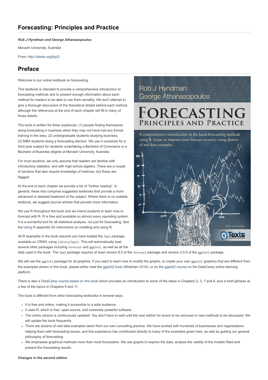
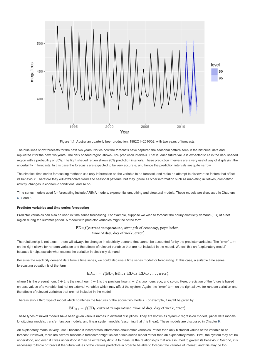
When forecasting time series data, the aim is to estimate how the sequence of observations will continue into the future. Figure 1.1 shows the quarterly
Australian beer production from 1992 to the second quarter of 2010.
�
Figure 1.1: Australian quarterly beer production: 1992Q1–2010Q2, with two years of forecasts.
The blue lines show forecasts for the next two years. Notice how the forecasts have captured the seasonal pattern seen in the historical data and
replicated it for the next two years. The dark shaded region shows 80% prediction intervals. That is, each future value is expected to lie in the dark shaded
region with a probability of 80%. The light shaded region shows 95% prediction intervals. These prediction intervals are a very useful way of displaying the
uncertainty in forecasts. In this case the forecasts are expected to be very accurate, and hence the prediction intervals are quite narrow.
The simplest time series forecasting methods use only information on the variable to be forecast, and make no attempt to discover the factors that affect
its behaviour. Therefore they will extrapolate trend and seasonal patterns, but they ignore all other information such as marketing initiatives, competitor
activity, changes in economic conditions, and so on.
Time series models used for forecasting include ARIMA models, exponential smoothing and structural models. These models are discussed in Chapters
6, 7 and 8.
Predictor variables and time series forecasting
Predictor variables can also be used in time series forecasting. For example, suppose we wish to forecast the hourly electricity demand (ED) of a hot
region during the summer period. A model with predictor variables might be of the form
The relationship is not exact—there will always be changes in electricity demand that cannot be accounted for by the predictor variables. The “error” term
on the right allows for random variation and the effects of relevant variables that are not included in the model. We call this an “explanatory model”
because it helps explain what causes the variation in electricity demand.
Because the electricity demand data form a time series, we could also use a time series model for forecasting. In this case, a suitable time series
forecasting equation is of the form
where is the present hour,
on past values of a variable, but not on external variables which may affect the system. Again, the “error” term on the right allows for random variation and
the effects of relevant variables that are not included in the model.
is two hours ago, and so on. Here, prediction of the future is based
is the next hour,
is the previous hour,
There is also a third type of model which combines the features of the above two models. For example, it might be given by
These types of mixed models have been given various names in different disciplines. They are known as dynamic regression models, panel data models,
longitudinal models, transfer function models, and linear system models (assuming that
is linear). These models are discussed in Chapter 9.
An explanatory model is very useful because it incorporates information about other variables, rather than only historical values of the variable to be
forecast. However, there are several reasons a forecaster might select a time series model rather than an explanatory model. First, the system may not be
understood, and even if it was understood it may be extremely difficult to measure the relationships that are assumed to govern its behaviour. Second, it is
necessary to know or forecast the future values of the various predictors in order to be able to forecast the variable of interest, and this may be too
E
D
=
f
(
c
u
r
r
e
n
t
t
e
m
p
e
r
a
t
u
r
e
,
s
t
r
e
n
g
t
h
o
f
e
c
o
n
o
m
y
,
p
o
p
u
l
a
t
i
o
n
,
t
i
m
e
o
f
d
a
y
,
d
a
y
o
f
w
e
e
k
,
e
r
r
o
r
)
.
=
f
(
,
,
,
,
…
,
e
r
r
o
r
)
,
E
D
t
+
1
E
D
t
E
D
t
−
1
E
D
t
−
2
E
D
t
−
3
t
t
+
1
t
−
1
t
−
2
=
f
(
,
c
u
r
r
e
n
t
t
e
m
p
e
r
a
t
u
r
e
,
t
i
m
e
o
f
d
a
y
,
d
a
y
o
f
w
e
e
k
,
e
r
r
o
r
)
.
E
D
t
+
1
E
D
t
f
�
difficult. Third, the main concern may be only to predict what will happen, not to know why it happens. Finally, the time series model may give more
accurate forecasts than an explanatory or mixed model.
The model to be used in forecasting depends on the resources and data available, the accuracy of the competing models, and the way in which the
forecasting model is to be used.
1.5 Some case studies
The following four cases are from our consulting practice and demonstrate different types of forecasting situations and the associated problems that often
arise.
Case 1
The client was a large company manufacturing disposable tableware such as napkins and paper plates. They needed forecasts of each of hundreds of
items every month. The time series data showed a range of patterns, some with trends, some seasonal, and some with neither. At the time, they were
using their own software, written in-house, but it often produced forecasts that did not seem sensible. The methods that were being used were the
following:
1. average of the last 12 months data;
2. average of the last 6 months data;
3. prediction from a straight line regression over the last 12 months;
4. prediction from a straight line regression over the last 6 months;
5. prediction obtained by a straight line through the last observation with slope equal to the average slope of the lines connecting last year’s and this
year’s values;
6. prediction obtained by a straight line through the last observation with slope equal to the average slope of the lines connecting last year’s and this
year’s values, where the average is taken only over the last 6 months.
They required us to tell them what was going wrong and to modify the software to provide more accurate forecasts. The software was written in COBOL,
making it difficult to do any sophisticated numerical computation.
Case 2
In this case, the client was the Australian federal government, who needed to forecast the annual budget for the Pharmaceutical Benefit Scheme (PBS).
The PBS provides a subsidy for many pharmaceutical products sold in Australia, and the expenditure depends on what people purchase during the year.
The total expenditure was around A$7 billion in 2009, and had been underestimated by nearly $1 billion in each of the two years before we were asked to
assist in developing a more accurate forecasting approach.
In order to forecast the total expenditure, it is necessary to forecast the sales volumes of hundreds of groups of pharmaceutical products using monthly
data. Almost all of the groups have trends and seasonal patterns. The sales volumes for many groups have sudden jumps up or down due to changes in
what drugs are subsidised. The expenditures for many groups also have sudden changes due to cheaper competitor drugs becoming available.
Thus we needed to find a forecasting method that allowed for trend and seasonality if they were present, and at the same time was robust to sudden
changes in the underlying patterns. It also needed to be able to be applied automatically to a large number of time series.
Case 3
A large car fleet company asked us to help them forecast vehicle re-sale values. They purchase new vehicles, lease them out for three years, and then
sell them. Better forecasts of vehicle sales values would mean better control of profits; understanding what affects resale values may allow leasing and
sales policies to be developed in order to maximize profits.
At the time, the resale values were being forecast by a group of specialists. Unfortunately, they saw any statistical model as a threat to their jobs, and
were uncooperative in providing information. Nevertheless, the company provided a large amount of data on previous vehicles and their eventual resale
values.
Case 4
In this project, we needed to develop a model for forecasting weekly air passenger traffic on major domestic routes for one of Australia’s leading airlines.
The company required forecasts of passenger numbers for each major domestic route and for each class of passenger (economy class, business class
and first class). The company provided weekly traffic data from the previous six years.
Air passenger numbers are affected by school holidays, major sporting events, advertising campaigns, competition behaviour, etc. School holidays often
do not coincide in different Australian cities, and sporting events sometimes move from one city to another. During the period of the historical data, there
was a major pilots’ strike during which there was no traffic for several months. A new cut-price airline also launched and folded. Towards the end of the
historical data, the airline had trialled a redistribution of some economy class seats to business class, and some business class seats to first class. After
several months, however, the seat classifications reverted to the original distribution.
1.6 The basic steps in a forecasting task
A forecasting task usually involves five basic steps.
Step 1: Problem definition.
�
Often this is the most difficult part of forecasting. Defining the problem carefully requires an understanding of the way the forecasts will be used, who
requires the forecasts, and how the forecasting function fits within the organization requiring the forecasts. A forecaster needs to spend time talking to
everyone who will be involved in collecting data, maintaining databases, and using the forecasts for future planning.
Step 2: Gathering information.
There are always at least two kinds of information required: (a) statistical data, and (b) the accumulated expertise of the people who collect the data
and use the forecasts. Often, it will be difficult to obtain enough historical data to be able to fit a good statistical model. However, occasionally, very
old data will be less useful due to changes in the system being forecast.
Step 3: Preliminary (exploratory) analysis.
Always start by graphing the data. Are there consistent patterns? Is there a significant trend? Is seasonality important? Is there evidence of the
presence of business cycles? Are there any outliers in the data that need to be explained by those with expert knowledge? How strong are the
relationships among the variables available for analysis? Various tools have been developed to help with this analysis. These are discussed in
Chapters 2 and 6.
Step 4: Choosing and fitting models.
The best model to use depends on the availability of historical data, the strength of relationships between the forecast variable and any explanatory
variables, and the way in which the forecasts are to be used. It is common to compare two or three potential models. Each model is itself an artificial
construct that is based on a set of assumptions (explicit and implicit) and usually involves one or more parameters which must be estimated using the
known historical data. We will discuss regression models (Chapter 5), exponential smoothing methods (Chapter 7), Box-Jenkins ARIMA models
(Chapter 8), Dynamic regression models (Chapter 9), Hierarchical forecasting (Chapter 10), and a variety of other topics including count time series,
neural networks and vector autoregression in Chapter 11.
Step 5: Using and evaluating a forecasting model.
Once a model has been selected and its parameters estimated, the model is used to make forecasts. The performance of the model can only be
properly evaluated after the data for the forecast period have become available. A number of methods have been developed to help in assessing the
accuracy of forecasts. There are also organizational issues in using and acting on the forecasts. A brief discussion of some of these issues is given in
Chapter 3.
1.7 The statistical forecasting perspective
The thing we are trying to forecast is unknown (or we wouldn’t be forecasting it), and so we can think of it as a random variable. For example, the total
sales for next month could take a range of possible values, and until we add up the actual sales at the end of the month, we don’t know what the value will
be. So until we know the sales for next month, it is a random quantity.
Because next month is relatively close, we usually have a good idea what the likely sales values could be. On the other hand, if we are forecasting the
sales for the same month next year, the possible values it could take are much more variable. In most forecasting situations, the variation associated with
the thing we are forecasting will shrink as the event approaches. In other words, the further ahead we forecast, the more uncertain we are.
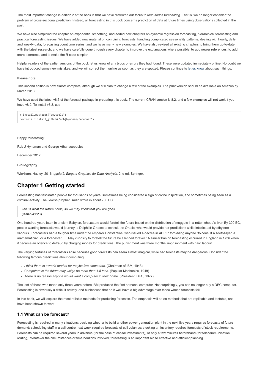
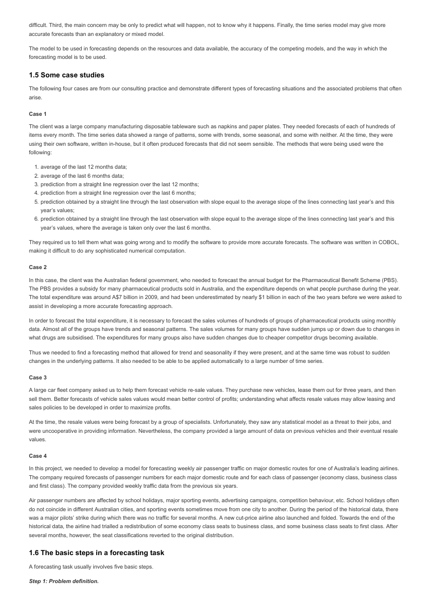
We can imagine many possible futures, each yielding a different value for the thing we wish to forecast. Plotted below in black are the total international
visitors to Australia from 1980 to 2015. Also shown are ten possible futures from 2016–2025.
�
Figure 1.2: Total international visitors to Australia (1980-2015) along with ten possible futures.
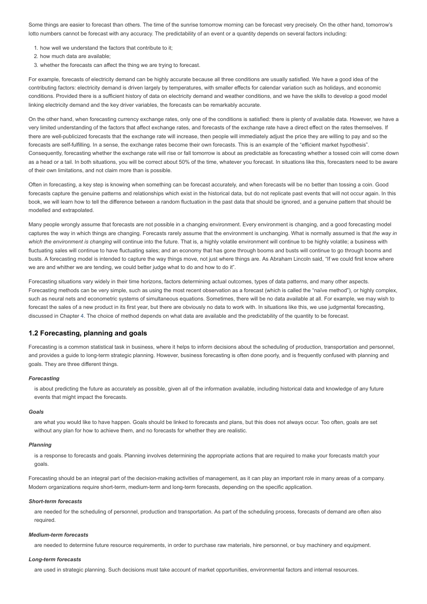
When we obtain a forecast, we are estimating the middle of the range of possible values the random variable could take. Very often, a forecast is
accompanied by a prediction interval giving a range of values the random variable could take with relatively high probability. For example, a 95%
prediction interval contains a range of values which should include the actual future value with probability 95%.
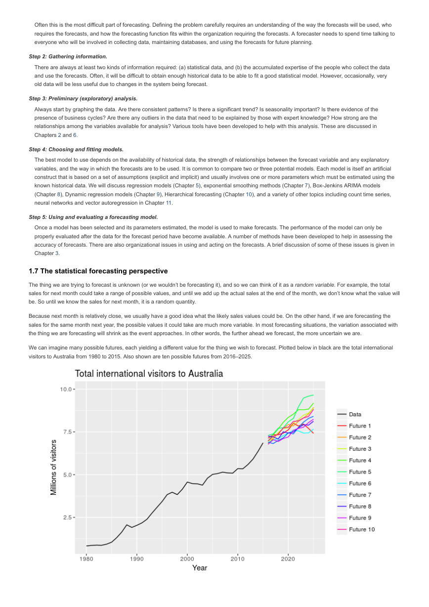
Instead of plotting individual possible futures as shown in Figure 1.2, we normally show these prediction intervals instead. The plot below shows 80% and
95% intervals for the future Australian international visitors. The blue line is the average of the possible future values, which we call the “point forecasts”.
Figure 1.3: Total international visitors to Australia (1980–2015) along with 10-year forecasts and 80% and 95% prediction intervals.
We will use the subscript for time. For example,
and we want to forecast
could take, along with their relative probabilities, is known as the “probability distribution” of
meaning “the random variable
. We then write
will denote the observation at time . Suppose we denote all the information we have observed as
”. The set of values that this random variable
given what we know in
. In forecasting, we call this the “forecast distribution”.
When we talk about the “forecast”, we usually mean the average value of the forecast distribution, and we put a “hat” over
the forecast of
the median (or middle value) of the forecast distribution instead.
, meaning the average of the possible values that
could take given everything we know. Occasionally, we will use
to show this. Thus, we write
to refer to
as
It is often useful to specify exactly what information we have used in calculating the forecast. Then we will write, for example,
of
step forecast taking account of all observations up to time
taking account of all previous observations
means the forecast of
. Similarly,
taking account of
).
to mean the forecast
-
(i.e., an
1.8 Exercises
1. For cases 3 and 4 in Section 1.5, list the possible predictor variables that might be useful, assuming that the relevant data are available.
2. For case 3 in Section 1.5, describe the five steps of forecasting in the context of this project.
1.9 Further reading
Armstrong (2001) covers the whole field of forecasting, with each chapter written by different experts. It is highly opinionated at times (and we don’t
agree with everything in it), but is full of excellent general advice on tackling forecasting problems.
Ord and Fildes (2012) is a forecasting textbook covering some of the same areas as this book, but with a different emphasis and not focussed around
any particular software environment. It is written by two of the most highly respected forecasters in the world, with many decades of experience
between them.
Bibliography
Armstrong, J S, ed. 2001. Principles of Forecasting: A Handbook for Researchers and Practitioners. Kluwer Academic Publishers.
Ord, J Keith, and Robert Fildes. 2012. Principles of Business Forecasting. South-Western College Pub.
t
y
t
t
I
y
t
|
I
y
t
y
t
I
|
I
y
t
y
y
t
y
^
t
y
t
y
^
t
y
^
t
|
t
−
1
y
t
(
,
…
,
)
y
1
y
t
−
1
y
^
T
+
h
|
T
y
T
+
h
,
…
,
y
1
y
T
h
T
�


 2023年江西萍乡中考道德与法治真题及答案.doc
 2012年重庆南川中考生物真题及答案.doc
 2013年江西师范大学地理学综合及文艺理论基础考研真题.doc
 2020年四川甘孜小升初语文真题及答案I卷.doc
 2020年注册岩土工程师专业基础考试真题及答案.doc
 2023-2024学年福建省厦门市九年级上学期数学月考试题及答案.doc
 2021-2022学年辽宁省沈阳市大东区九年级上学期语文期末试题及答案.doc
 2022-2023学年北京东城区初三第一学期物理期末试卷及答案.doc
 2018上半年江西教师资格初中地理学科知识与教学能力真题及答案.doc
 2012年河北国家公务员申论考试真题及答案-省级.doc
 2020-2021学年江苏省扬州市江都区邵樊片九年级上学期数学第一次质量检测试题及答案.doc
 2022下半年黑龙江教师资格证中学综合素质真题及答案.doc