A Joint Algorithm of Parameters Estimation for Frequency-Hopping Signal Based on Sparse Recovery Xiaolin Zhang, Xiaofang Hu, Xue Dong College of Information and Communication Engineering Harbin Engineering University Harbin, China Email: huxiaofang36@hrbeu.edu.cn Abstract— Parameters estimation is a crucial and challeng- ing component for Frequency-Hopping (FH) communication. Time-frequency analysis is a valid signal processing tool to estimate parameters of FH signal. However, the existing Time-Frequency analysis methods have several shortcomings such as weak suppression noise interference and feeble concentration of Time-Frequency, resulting in inaccurate parameter estimation. To tackle these challenges, we propose a novel joint algorithm by incorporating the approximation of L0 norm (AL0) and sparse linear regression (SLR). In detail, AL0 is used to obtain accurate frequency sets from the Time-Frequency representation, and SLR is used to estimate the hop period, combined with the frequency sets got from AL0 algorithm. Finally, an accurate estimation of the frequency hopping pattern is achieved. Simulation results demonstrate that the joint algorithm can effectively obtain the frequencies and hop period. Besides, the joint algorithm outperforms the SLR algorithm in estimating the period with low Signal Noise Ratio (SNR). Finally accurately recover the FH pattern. Keywords – FH signal; parameter estimation; approximation L0 norm(AL0); sparse linear regression(SLR); FH pattern. I. INTRODUCTION Parameter estimation of FH signal is an essential prob- lem with applications in both military and civilian do- mains. Time-Frequency analysis is widely adopted in the parameter estimation of FH signals. At present, Time- Frequency analysis methods include Short-Time Fourier Transform (STFT), Wigner-Ville Distribution (WVD), S- mooth Pseudo-Wigner-Ville Distribution (SPWVD) and so on. Estimation accuracy of STFT depends heavily on the size of window, and there is a conflict between time domain and frequency domain resolution [1-2]. Compared with STFT, WVD has a higher Time-Frequency resolution, but there are cross-term interferences [3]. SPWVD is proposed on the basis of WVD, and it reduces the cross- term interferences by the time domain and frequency domain windowing, while SPWVD limits its application in practice with a large amount of calculation [4]. At the side of STFT, WVD and SPWVD, the AL0 algorithm can get a more clear and concentrated Time-Frequency repre- sentation in a lower SNR [5-6]. However, the jump time performance is coarse for the limitation of the principle, with the error can be accepted in a certain limited range. The SLR algorithm can estimate period exactly, because it reconstructs the FH signal with a complete frequency sets, which makes a computational burden [7-9]. In reality, parameter estimation with high precision can’t achieved by single method. To solve this problem, a novel joint algorithm utilizing AL0 and SLR is proposed. Firstly, the FH signal is processed by AL0 and the frequency sets is estimated exactly. Secondly, the frequency sets is processed with SLR to obtain the hop period. Finally, the FH pattern is recovered based on the frequency and period. Simulation results show that the joint algorithm can estimate the jump period more accurately and recovery FH pattern efficiently. II. PROBLEM FORMULATION A. Frequency-Hopping Signal Model It is assumed that only one FH signal is received, signal model can be described as follows [10] y(t) = s(t) + υ(t) K = k=1 (1) TH ) + υ(t), + φk)]rect( t ak exp[j(2πfkt = t − (k − 1)TH − αTH , s(t) denotes the where t FH signal, v(t) is additive noise, rect(t) represents a rectangular window, TH is jump period. There are K jumps in the observation time, ak is amplitude, fk is frequency, φk is the initial phase, and initial jump duration is αTH. As we all know, the FH signal is sparse, thus suppose that the signal s ∈ C P is k sparse on a set of orthogonal frequency bases Ψ = [Ψ1, Ψ2,··· , ΨP ] ∈ C P×P , the FH signal can be expressed as P i=1 s = Ψiαi or s = Ψα, (2) where α ∈ C P contains k nonzero coefficients corre- sponding to the active frequency, take into account the influence of noise, the model in (1) can be rewritten as y = Ψα + υ. (3) 978-1-5386-2062-5/17/$31.00 ©2017 IEEE 

is mutated [12]. Therefore, the AL0 algorithm is used to introduce the Gaussian function to approximate the l0 norm [13] : fδ(s) = 1 − exp(− s2 2δ2 ), (11) when δ approaches 0, then f (si) ≈ s0 . N i=1 P , For single observation, denote Fδ(xk) = Fδ(xk) = xk0. Similarly, then lim δ→0 fδ(xik) i=1 for multi- Fδ(ζ) = ζ0 observation Fδ(ζ) = . Consequently, the model in (10) can be represented as : fδ(ζi) , then lim δ→0 P i=1 L(X)= [yk − Wxk2 2 + μ1 fδ(xik)]+μ2 fδ(ζi) P i=1 P i=1 K k=1 (7) (12) The Time-Frequency matrix X can be estimated by solv- ing the model (12). B. The Theory of Approximation of L0 Norm Suppose that the frequency of the received FH signal {ωk} belongs to a known finite frequency sets W = {ω1, ω2,··· , ωP} , namely {ωk} ⊂ W . Let W denotes the matrix which is composed by Fourier orthogonal bases [11] W = [ω0,ω1,··· ,ωP−1] ωi = [ejωi1, ejωi2,··· , ejωiP T . ] (4) (5) Divide the received signal y into K segments, where yi is composed of columns to form the data observation matrix Y Y = [y0, y1,··· , yK−1], (6) where yi = y(iL : iL + P − 1), P is the length of the segment, and L represents the interval, namely, L = round((N − P )/K) . The model in (3) can be reconstruct as Y = WX + V, X depicts the Time-Frequency distribution of the FH signal, it is made up with 0 and 1. V represents the noise matrix and X, V ∈ C P×K . According to the Time-Frequency sparse property of the FH signal, X is sparse. Thus, in order to solve the X , unconstrained optimization function with penalty function can constructed as below: L(X) = Y − WX2 F + μ1X0 + μ2X2,0 (8) ˆX = arg min X∈CP×K [L(X)], μ1, μ2 are penalty factor, which belong to the point sparse and the row joint sparse of the X , respectively. The value of μ1, μ2 should be appropriate, small value will weaken the noise suppression ability and bigger value will impair the amplitude of the true signal. The reference [5] has demonstrated the suitable value of penalty factor in detail, in generally μ1=P/4 , μ2 = P . The first term •2 F represents the F- norm, the second term embodies the sparse reconstruction problem of single observation, and the third term indicates a multi-observation joint sparse situation. Let X(i, :) represents i-th row of the X, and the lp,q norm is defined as : Xp,q = ( K K Thus, the model in (8) can be rewritten as Y(:, k)−WX(:, k)2 X(:, k)0+μ2ζ0 (X(i, :)p) N L(X)= +μ1 (10) (9) k=1 i=1 q . ) 2 q 1 k=1 where ζ = [ζ1, ζ2,··· , ζP ]T and ζi = X(i, :)2, i = 1, 2,··· , P . As we all know that the optimization problem showed in (10) is difficult to solve directly, because the zero norm C. The Theory of Sparse Linear Regression Suppose that the frequency sets of the FH signal {ωk} belong to a known finite sets W = {ω1, ω2,··· , ωP}, so, the signal can be shown as a linear function of the W , yn = ωn T xn + υn, n ∈ {0, 1, . . . , N − 1} (13) where ωn = [ejω1n, ejω2n, . . . , ejωP n]T ∈ CP×1 , ωn represents the frequency sets at n time, xn = [xn,1, xn,2, . . . , xn,P ]T ∈ CP×1 , xn,p represents the amplitude and phase of the p-th frequency bin at time n [7-8]. Denoting: X∗ 0 , xT = [xT 1 , . . . , xT T ∈ CP×1 N−1] T ∈ CN×P N W = [w0, w1, . . . , wN−1] T ∈ CP N×1 P , . . . 0T P N−n−1 the FH signal can be constructed as wn = [0T P , . . . 0T P n , 0T , ωT n ] (14) (15) (16) Y = WX∗ (17) The matrix X∗ can be obtained by the augmented La- grange method as follows [8]: +V L(X, Z, U,ζ, μ) = 2 + λ1Z1 + λ2U1 (DX − μ)} (X − Z) + μH Y − WX2 1 2 +{ζH c + (X − Z2 2 + DX − U2 2), 2 (18) where D = [dT 1 , dT (1) 1 ,··· , dT ((N−1)P−1) 1 1 = [−1, 0, . . . 0 dT P−1 , 1, 0, . . . 0 (N−1)P−1 ] T ∈ R(N−1)P×N P (19) (20) T ] 

Fig. 1. Process diagram of Frequency-Hopping signal The (•)m represents the right cyclic shift of m position. ζ, μ are Lagrange multipliers, coefficient matrix X can be estimated by solving the equation (18). A. Parameters Estimation Scheme of Frequency-Hopping Signal We have learnt that the SLR algorithm can estimate period exactly with a complete frequency sets, which makes a computational burden. It’s worth mentioning that AL0 algorithm can precisely estimate the frequency with a relatively smaller amount of calculation. In view of this, a now joint algorithm is proposed and the estimation scheme of FH pattern can be described as Fig.1. B. The Process to Obtain Time-Frequency Matrix in Ap- proximation of L0 Norm Algorithm In this paper, the steepest descent algorithm is used to solve the X . The steepest descent direction is the conjugate gradient direction of the objective function. The conjugate gradient of model (12) is ∇L(X) = WH μ2Λ2X (21) (x) = exp(− x2 where, Λ1 = fδ 2δ2 ) , Λ2 is a diagonal matrix, whose diagonal element is exp(−X(n, :)2 2 /2δ2)/δ2, X(n, :) represents the n-th row of the matrix. (WX − Y) + μ1Λ1• ∗ X + (X)/δ2 , and fδ 1 2 1 2 The AL0 algorithm can be divided into the following −1Y ; steps: 1. The initial value of X is X(0)=WT(WWT) III. JOINT ALGORITHM μ(i) 2. Select a set of descending sequence [δ1, δ2,··· , δJ ] [13], the convergence criterion is ε ; 3. Denote δ = δj and j = 1, 2,··· , J , the algorithm iterates over the following steps: 1) Determine the step size u Lδ(X − u∇L(X)) < Lδ(X) temp1 = norm(X). 2) Descend in the gradient direction X = X − u∇L(X) temp2 = norm(X) 3) The iteration termination condition if dif f (abs(temp2 − temp1)) < ε , execute X(j) = X 4) Output the results ˆX = X(J) . C. The Process to Obtain Time-Frequency Matrix in S- parse Linear Regression Algorithm In this paper, we use the alternating direction method of multipliers (ADMOM) method to solve the (18) to get X , and the ADMOM iterates over the following steps (WH Y − ζ(i−1) =(WHW + cDH D + cINP) X(i) −1 − DH μ(i−1) + cZ(i−1) Z(i) = shrink(X(i) + U(i) = shrink(DX(i) + cDH U(i−1) ζ(i−1) , λ1 c ) c μ(i−1) ) (22) (23) (24) (25) (26) λ2 c ) ). c + , + c(X(i) − Z(i) ) + c(DX(i) − U(i) , Z(0) 2 ζ(i) = ζ(i−1) = μ(i−1) 2 X(i) / 2 the initial vectors X(0) X(i) − X(i−1) Where, , μ(0) are arbitrary, the iteration termination condition is < ε , and the shrinkage ,U(0) ,ζ(0) 2 operator is: shrink(x, y) = 0 x = 0 x|x| max(|x| − y, 0), otherwish. , if (27) IV. SIMULATION Simulation conditions: the number of the grid frequency is P = 60 , thus the complete frequency sets are W = {2π p P }×1KHz, p = 1, 2,··· , P , frequency of each jump are [W (20), W (12), W (18), W (7)] , length of the signal processed is N = 800 sampling points in this thesis, and the hop period is 200 points. 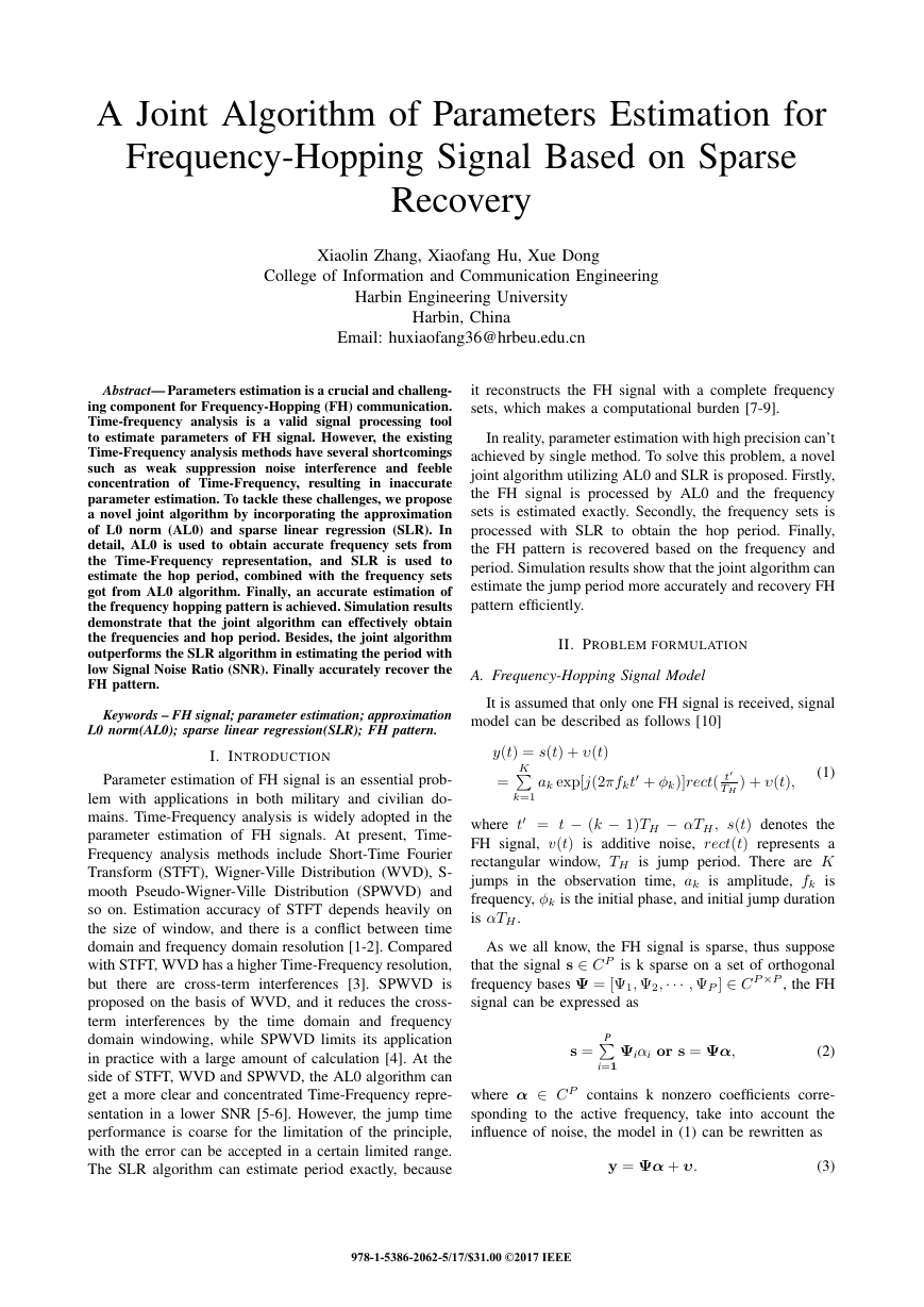In Fig.2 (a), (c), (e) shows the performance of different algorithm with 0dB, and (b), (d), (f) with -5dB. It can be seen that the results of the STFT is greatly affected by the noise. The effect of SPWVD is better, but the Time- Frequency resolution is feeble. Compared with these two algorithms, we can apparently see that AL0 is less affect by noise, and the Time-Frequency resolution is high even at -5dB, the performance is better at 0dB. 

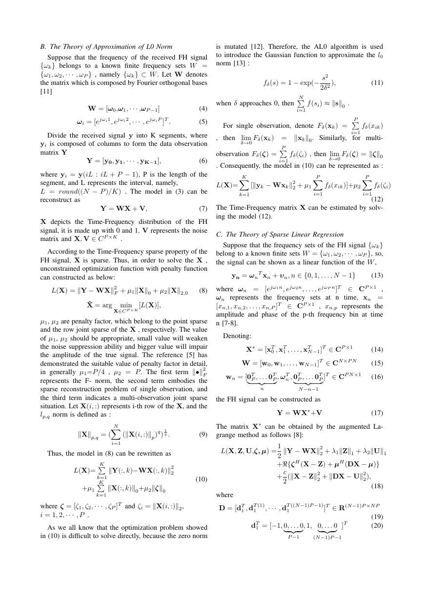
(a) STFT with 0 dB (b) STFT with -5 dB (c) SPWVD with 0 dB (d) SPWVD with -5 dB (e) AL0 with 0 dB (f) AL0 with -5 dB Fig. 2. The estimation of Time-Frequency representation The Table 1 lists the relative error of the frequency, which is estimated from the Time-Frequency representa- tion obtained above. It manifests that AL0 can precisely estimate the frequency at 0dB, however, the estimation of STFT and SPWVD is coarse. 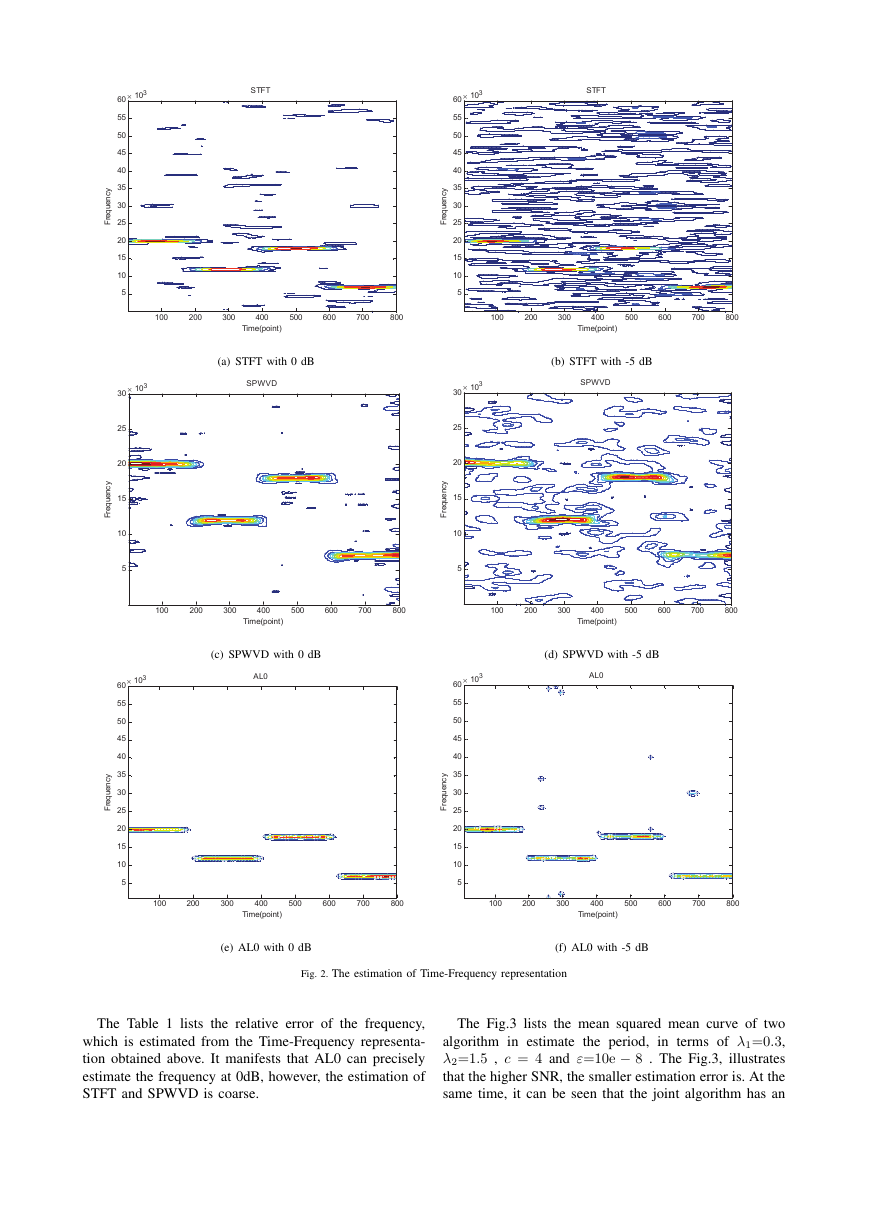The Fig.3 lists the mean squared mean curve of two algorithm in estimate the period, in terms of λ1=0.3, λ2=1.5 , c = 4 and ε=10e − 8 . The Fig.3, illustrates that the higher SNR, the smaller estimation error is. At the same time, it can be seen that the joint algorithm has an 

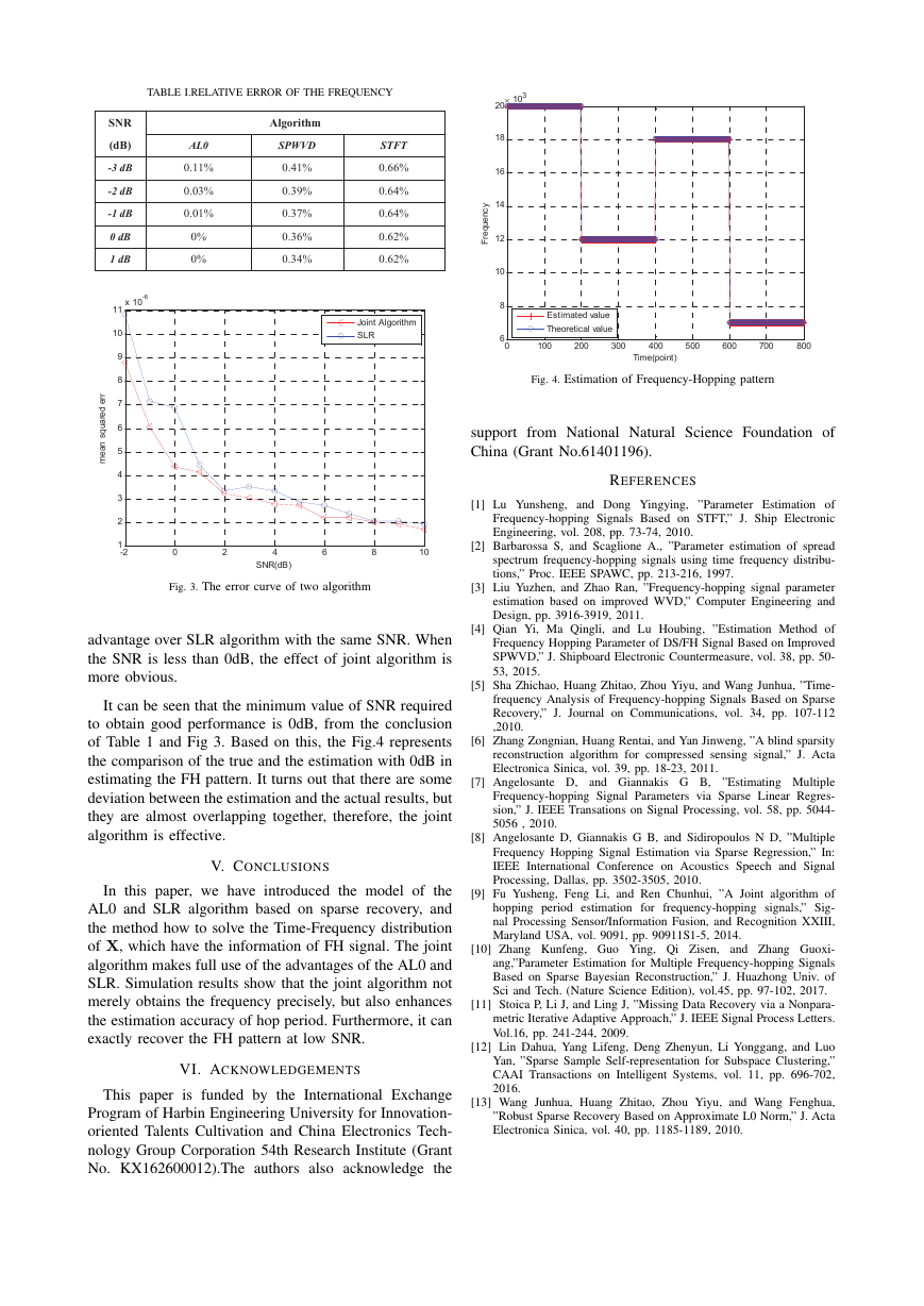
TABLE I.RELATIVE ERROR OF THE FREQUENCY Fig. 3. The error curve of two algorithm advantage over SLR algorithm with the same SNR. When the SNR is less than 0dB, the effect of joint algorithm is more obvious. It can be seen that the minimum value of SNR required to obtain good performance is 0dB, from the conclusion of Table 1 and Fig 3. Based on this, the Fig.4 represents the comparison of the true and the estimation with 0dB in estimating the FH pattern. It turns out that there are some deviation between the estimation and the actual results, but they are almost overlapping together, therefore, the joint algorithm is effective. V. CONCLUSIONS In this paper, we have introduced the model of the AL0 and SLR algorithm based on sparse recovery, and the method how to solve the Time-Frequency distribution of X, which have the information of FH signal. The joint algorithm makes full use of the advantages of the AL0 and SLR. Simulation results show that the joint algorithm not merely obtains the frequency precisely, but also enhances the estimation accuracy of hop period. Furthermore, it can exactly recover the FH pattern at low SNR. VI. ACKNOWLEDGEMENTS This paper is funded by the International Exchange Program of Harbin Engineering University for Innovation- oriented Talents Cultivation and China Electronics Tech- nology Group Corporation 54th Research Institute (Grant No. KX162600012).The authors also acknowledge the Fig. 4. Estimation of Frequency-Hopping pattern support from National Natural Science Foundation of China (Grant No.61401196). REFERENCES [1] Lu Yunsheng, and Dong Yingying, ”Parameter Estimation of Frequency-hopping Signals Based on STFT,” J. Ship Electronic Engineering, vol. 208, pp. 73-74, 2010. [2] Barbarossa S, and Scaglione A., ”Parameter estimation of spread spectrum frequency-hopping signals using time frequency distribu- tions,” Proc. IEEE SPAWC, pp. 213-216, 1997. [3] Liu Yuzhen, and Zhao Ran, ”Frequency-hopping signal parameter estimation based on improved WVD,” Computer Engineering and Design, pp. 3916-3919, 2011. [4] Qian Yi, Ma Qingli, and Lu Houbing, ”Estimation Method of Frequency Hopping Parameter of DS/FH Signal Based on Improved SPWVD,” J. Shipboard Electronic Countermeasure, vol. 38, pp. 50- 53, 2015. [5] Sha Zhichao, Huang Zhitao, Zhou Yiyu, and Wang Junhua, ”Time- frequency Analysis of Frequency-hopping Signals Based on Sparse Recovery,” J. Journal on Communications, vol. 34, pp. 107-112 ,2010. [6] Zhang Zongnian, Huang Rentai, and Yan Jinweng, ”A blind sparsity reconstruction algorithm for compressed sensing signal,” J. Acta Electronica Sinica, vol. 39, pp. 18-23, 2011. and Giannakis G B, ”Estimating Multiple Frequency-hopping Signal Parameters via Sparse Linear Regres- sion,” J. IEEE Transations on Signal Processing, vol. 58, pp. 5044- 5056 , 2010. [7] Angelosante D, [8] Angelosante D, Giannakis G B, and Sidiropoulos N D, ”Multiple Frequency Hopping Signal Estimation via Sparse Regression,” In: IEEE International Conference on Acoustics Speech and Signal Processing, Dallas, pp. 3502-3505, 2010. [9] Fu Yusheng, Feng Li, and Ren Chunhui, ”A Joint algorithm of hopping period estimation for frequency-hopping signals,” Sig- nal Processing Sensor/Information Fusion, and Recognition XXIII, Maryland USA, vol. 9091, pp. 90911S1-5, 2014. [10] Zhang Kunfeng, Guo Ying, Qi Zisen, and Zhang Guoxi- ang,”Parameter Estimation for Multiple Frequency-hopping Signals Based on Sparse Bayesian Reconstruction,” J. Huazhong Univ. of Sci and Tech. (Nature Science Edition), vol.45, pp. 97-102, 2017. [11] Stoica P, Li J, and Ling J, ”Missing Data Recovery via a Nonpara- metric Iterative Adaptive Approach,” J. IEEE Signal Process Letters. Vol.16, pp. 241-244, 2009. [12] Lin Dahua, Yang Lifeng, Deng Zhenyun, Li Yonggang, and Luo Yan, ”Sparse Sample Self-representation for Subspace Clustering,” CAAI Transactions on Intelligent Systems, vol. 11, pp. 696-702, 2016. [13] Wang Junhua, Huang Zhitao, Zhou Yiyu, and Wang Fenghua, ”Robust Sparse Recovery Based on Approximate L0 Norm,” J. Acta Electronica Sinica, vol. 40, pp. 1185-1189, 2010.