4834
IEEE TRANSACTIONS ON IMAGE PROCESSING, VOL. 24, NO. 12, DECEMBER 2015
Image Outlier Detection and Feature Extraction via
L1-Norm-Based 2D Probabilistic PCA
Fujiao Ju, Yanfeng Sun, Junbin Gao, Yongli Hu, and Baocai Yin
paper
an
introduces
Abstract— This
L1-norm-based
probabilistic principal
component analysis model on 2D
data (L1-2DPPCA) based on the assumption of the Laplacian
noise model. The Laplacian or L1 density function can be
expressed as a superposition of an infinite number of Gaussian
distributions. Under this expression, a Bayesian inference can be
established based on the variational expectation maximization
approach. All the key parameters in the probabilistic model
can be learned by the proposed variational algorithm. It has
experimentally been demonstrated that the newly introduced
hidden variables in the superposition can serve as an effective
indicator for data outliers. Experiments on some publicly
available databases show that the performance of L1-2DPPCA
has largely been improved after identifying and removing
sample outliers, resulting in more accurate image reconstruction
than the existing PCA-based methods. The performance of
feature extraction of the proposed method generally outperforms
other existing algorithms in terms of reconstruction errors and
classification accuracy.
Index Terms— L1-norm, probabilistic principal component
analysis, variational Bayesian inference, outlier detection, feature
extraction.
I. INTRODUCTION
H IGH-DIMENSIONAL and multiple array data are
widely acquired in modern computer vision research.
This high-dimensionality of data not only increases computa-
tional overhead and memory requirements in algorithms, but
also adversely affects their performance in real applications.
However, high-dimensional data are not often distributed uni-
formly in their ambient space, instead they lie in or close to a
low-dimensional space or manifold [23], [33]. Finding the low-
dimensional embedding for high-dimensional observed data
has been a challenging problem in machine learning research.
However, much progress has been made towards building tools
or algorithms for dimensionality reduction in the last couple
of decades [3], [8], [11], [17].
Principle Component Analysis (PCA) [2] is one of popular
dimensionality reduction methods widely used in image
analysis [7], [10], pattern recognition [6], [18] and machine
learning [13] for data analysis. PCA can be interpreted in
many ways, one of which assumes that the observed high-
dimensional data are generated from their low-dimensional
factors through a linear model with the corruption of Gaussian
noise, i.e., measured by the L2-norm. Traditional PCA is
concerned with vectorial data and has been very successful
in applications [13], [28]. Today data emerging from science
and technology are in new types with more structures. For
example, image data should be regarded as 2D tensors in
order to preserve their 2D spatial information. In order to
apply the classical PCA to such 2D image data, a typical
workaround is to vectorize 2D data. Vectorizing 2D data not
only preserves the high-dimensionality of data, causing the
problem of the curse of dimensionality [25], but also ignores
valuable information about the spatial relationships among
2D data.
for
Further,
feature extraction or
the data-as-vector PCA approach will be sub-
optimal
representation because
of spatial information loss. Instead of using vectorization,
PCA approaches for two-dimensional data (2DPCA) have been
proposed [24], [27]. Compared with the traditional PCA,
2DPCA directly conducts analysis on 2D data matrices so that
the structural relation between data entries can be preserved
and more spatial information can be utilized [12], [20], [30].
Numerous experiments have shown that 2DPCA with less
parameters can achieve competitive or even better recognition
performance than PCA, especially when the sample size is
small relative to feature dimensionality. Similar to the conven-
tional PCA, 2DPCA models are also based on the L2-norm
error measurement.
Manuscript received December 31, 2014; revised May 27, 2015; accepted
August 7, 2015. Date of publication August 17, 2015; date of current
version September 18, 2015. This work was supported in part by the Natural
Science Foundation of Beijing, China, under Grant 4132013,
in part by
the Australian Research Council Discovery Projects Funding Scheme under
Grant DP130100364, and in part by the National Natural Science Foundation
of China, under Grant 61171169, Grant 61133003, Grant 61370119, and
Grant 61390510. The associate editor coordinating the review of this manu-
script and approving it for publication was Dr. Christopher Wyatt.
F.
Ju, Y. Sun, Y. Hu, and B. Yin are with the Beijing Key
Laboratory of Multimedia and Intelligent Technology, College of Metropolitan
Transportation, Beijing University of Technology, Beijing 100124, China
(e-mail:
jufujiao2013@emails.bjut.edu.cn; yfsun@bjut.edu.cn; huyonglig@
bjut.edu.cn; ybc@bjut.edu.cn).
J. Gao is with the School of Computing and Mathematics, Charles Sturt
University, Bathurst, NSW 2795, Australia (e-mail: jbgao@csu.edu.au).
Color versions of one or more of the figures in this paper are available
online at http://ieeexplore.ieee.org.
Digital Object Identifier 10.1109/TIP.2015.2469136
There exist a number of models for deriving PCA, the
majority of which are algebraic. Algebraic models don’t have
the flexibility of providing confidence information of the
model when dealing with noisy data. To combat this drawback,
Tipping and Bishop [22] proposed a probabilistic PCA model,
called PPCA. In PPCA, observed data are regarded as random
variables, generated from a set of latent random variables
which follow the Gaussian distribution of zero mean and
identity covariance, with additive noises following a Gaussian
distribution with zero mean and an isotropic covariance.
PPCA is a special case of the standard factor analysis (FA)
model [2] whose noise follows Gaussian distribution with
zero mean and diagonal covariance. Under the probabilistic
learning framework, the model parameters in PPCA can be
easily solved by the maximum likelihood estimation (MLE).
1057-7149 © 2015 IEEE. Personal use is permitted, but republication/redistribution requires IEEE permission.
See http://www.ieee.org/publications_standards/publications/rights/index.html for more information.
�
JU et al.: IMAGE OUTLIER DETECTION AND FEATURE EXTRACTION VIA L1-NORM-BASED 2D PROBABILISTIC PCA
4835
Furthermore, PPCA can be used to deal with the cases
containing missing values within the observed data, while the
traditional PCA is not valid in missing value cases. Recently,
Zhao et al. [34] proposed a probabilistic principle component
analysis model on 2D data, called 2DPPCA, which takes a
step forward for PPCA model in 2D cases.
A Gaussian noise distribution is assumed in both the afore-
mentioned PCA (implicitly) and PPCA (explicitly) methods.
However real-life data often contain noises which may not
follow Gaussian distributions, particularly in the cases of
existing outliers such as partial occlusion in scene images.
In such cases, both PCA and PPCA may produce a biased
model for data as the model will try to fit data under the
Gaussian noise assumption.
It has been well known that
the Laplacian distribution
(or L1 distribution) is less sensitive to outliers compared with
the Gaussian distribution. So it is a natural development to use
L1-norm as the error metric to replace the L2-norm measure-
ment used in both PCA and PPCA methods. There have been
many approaches proposed to include L1-norm or L1 dis-
tribution in an attempt to deal with data outliers. To the
best of our knowledge, Zhong and Zhang [36] proposed a
robust LDA instead of conventional LDA using L2-norm.
Baccini et al. [1] proposed the first L1-norm PCA (L1-PCA)
model. Meng et al. [19] proposed an L1-PCA model by max-
imizing the so-called L1 dispersion, while Ke and Kanade [9]
formulated L1-PCA by maximum likelihood estimation. They
use either heuristic estimate or weighted median method
and convex programming to obtain the projection matrix of
L1-PCA.
All of
in the alge-
braic framework with expensive computational cost and no
invariance to rotations. Aiming to diminish this drawback,
Kwak [14] proposed a fast and robust L1-norm PCA method,
termed as PCA-L1. Similar to [19], PCA-L1 replaces maxi-
mizing L2-norm based variance with L1-norm dispersion in
the feature space to realize robust and rotation invariant PCA.
Ding et al. [4] further extended L1-norm PCA to the R1-norm
(a modified L1-norm) based PCA (R1-PCA). It combines the
merits of L2-PCA and L1-PCA. The model is guaranteed to
be rotational invariant, however the convergent speed of the
algorithm is relatively slow. Li et al. [16] investigated the
implementation of fast PCA-L1 [14] for 2D data by simply
considering PCA-L1 model on multiple phases of 1D data
from 2D data. This method is robust to outliers because of
utilizing the L1-norm errors metric, and more information
regarding spatial relationships can be preserved.
the above mentioned models fall
Concerned with a probabilistic model for L1-PCA, Gao [5]
introduced a robust probabilistic L1-PCA model, called
L1-PPCA. In order to provide an effective learning algorithm,
the author expanded the Laplacian distribution as a superpo-
sition of infinite number of Gaussiann distributions so that
this model can be solved by using variational Expectation
Maximization (EM)-type algorithms.
Motivated by L1-PPCA, we propose a probabilistic
PCA model for 2D data (L1-2DPPCA) in this paper. The con-
tributions of the paper are three-fold. Firstly, in generalizing
L1-PPCA for 2D data, we formulate the error distribution in
terms of the Hadamard product to facilitate the variational
EM algorithm in dealing with the difficulty imposed by
using the multiple linear model, referring to equation (1).
Secondly, an analysis is given as the foundation for proposing
an indicator for outlier detection or identification, and finally
a strategy of using Gaussian distribution as approximated
posterior for the latent feature variables is proposed to over-
come the difficulty of non-Gaussian posterior in the variational
EM algorithm.
L1-2DPPCA has three major advantages: 1) The model
makes use of structural information within 2D data and can be
easily extended for high order tensorial data. All the algorithm
derivations remain without any major difficulty. 2) The model
is robust to grossly noises such as occlusion in images and can
be used as a stable outlier detector. It can be also generalized
to other noise models like student-t distribution. And 3) The
model uses less parameters than the vectorized L1-PPCA, thus
it requests less data for training.
the paper
is organized as follows.
In Section II, L1-2DPPCA model is introduced. The vari-
ational approximation technology for solving L1-2DPPCA
model is derived and presented in Section III and Appendix.
In Section IV, some experimental results are presented for
evaluating the performance of the proposed model. Finally,
conclusions are summarized in Section V.
The remainder of
II. L1-2DPPCA MODEL
Let X = {X1, X2, . . . , XN} be N independent and iden-
tically distributed random variables with values in Rm×n.
The probabilistic second-order PCA (PSOPCA) [32] is based
on the matrix-variate normal assumption and assumes the
following two-sides latent variable model:
Xk = LZkRT + M + Ek,
(1)
where L in size m × r and R in size n × c are the row and
column loading matrices, and Zk is the latent core variable
of Xk, with r (≤ m) rows and c (≤ n) columns, respectively.
M and Ek both in size m × n are the mean matrix and
the error matrix, respectively. Zk is regarded as the latent
representation of the observed data Xk, so the model can be
used as a feature extractor or dimensionality reduction through
a Bayesian inference process.
as
the
the
article
Without loss of generality, suppose M is a zero matrix
input data X can be
throughout
learning. Denote by N (X|M, U, V)
centralized in model
the matrix-variate Gaussian distribution with the mean M
and row covariance U and column covariance V [26].
If Ek ∼ N (Ek|0, σ Im , σ In),
i.e., for each error compo-
nents �i j ∼ N (�i j|0, σ 2)(i = 1, 2, . . . , m; j = 1, 2, . . . , n),
then model
probabilistic
2DPCA [31].
standard
leads
(1)
to
the
Although the conventional PCA based on L2-norm has
been successful for many applications, it is vulnerable to the
presence of outliers, because the effect of the outliers with
a large norm is exaggerated by the use of L2-norm. Outliers
exist widely, perhaps representing corrupted observations or
genuine samples from a heavy-tailed noise process. To cope
�
4836
IEEE TRANSACTIONS ON IMAGE PROCESSING, VOL. 24, NO. 12, DECEMBER 2015
with outliers in a 2D data set and estimate model confidence
levels, we introduce an L1-norm based 2D probabilistic PCA,
noted by L1-2DPPCA. We consider that the error component
�i j
is independent and identically distributed according to
a centered Laplacian distribution whose density function is
given by
pL1
(�|σ ) = 1
2σ
exp
− 1
σ
|�|
.
(2)
1
pL1
Based on the above equation, the joint distribution of all the
components of Ek can be written as, due to the independence
of the error component,
(Ek|σ ) =
(2σ )mn exp
|.
|e(k)
n
j=1
where Ek1 =
− 1
σ
Ek1
To develop a generative Bayesian model, we define a
Gaussian prior distribution p(Zk) over the latent variable.
Specifically, the prior distribution over Zk is given by the
following zero-mean unit-covariance matrix-variate Gaussian
distribution:
p(Zk) = N (Zk|0, Ir , Ic) =
rc
tr(ZT
m
i=1
exp
(3)
i j
,
.
2
k Zk )
− 1
2
1
2π
To model noise levels, we impose a prior Gamma distribu-
tion on ρ = 1/σ 2 instead of directly on σ in equation (3):
(4)
ρ
ρaρ−1exp{−bρρ}.
pσ (ρ) = �(ρ|aρ , bρ) = baρ
�(aρ )
(5)
For the sake of convenience, let Z = {Z1, . . . , ZN} denote
the model hidden variables, and � collect all
the model
parameters L and R, etc.
For the given observation X , the log likelihood can be
defined by its marginalized log likelihood over the assumed
latent variables Z and ρ
L(�) = log p(X|�) = log
p(X , Z, ρ|�)dZdρ.
(6)
ρ
Z
Then the learning task is
to learn model parameters
� (� = {L, R}) such that p(X|�) in (6) is maximized. A gen-
eral approach is to use the EM algorithm [2], where we need
to calculate the posterior over latent variables p(Z, ρ|X , �)
in the E-step and estimate model parameters � in the M-step.
the unknowns is, by
The posterior distribution over all
applying Bayes’ rule,
,
p(Z, ρ|X , �) = p(X , Z, ρ|�)
p(X|�)
(7)
where p(X , Z, ρ|�) is the joint distribution of the data set X ,
the latent variable Z, and the hidden parameters ρ. Under the
model assumptions (3), (4) and (5), the joint distribution is
given by
p(X , Z, ρ|�) = N
Unfortunately, we cannot compute the posterior analytically
as the denominator p(X|�) in (7) necessitates an intractable
(Xk − LZkRT|σ ) p(Zk) pσ (ρ).
k=1
pL1
(8)
integration due to the Laplacian distribution pL1. A direct
application of EM is not feasible. Therefore, we propose a
variational approximation scheme in the next section.
III. VARIATIONAL APPROXIMATION FOR L1-2DPPCA
Under the variational EM framework, instead of using the
exact posterior (7) in the EM algorithm, one uses an approx-
imated distribution Q(Z, ρ), called variational distribution,
over the hidden variables. For any distribution Q(Z, ρ), the
following lower bound on L(�) is guaranteed:
p(X , Z, ρ|�)dZdρ
L(�) = log
≥
Z
ρ
−
Z
ρ
Q(Z, ρ)log p(X , Z, ρ|�)dZdρ
Q(Z, ρ)logQ(Z, ρ)dZdρ
Z
ρ
F (Q(Z, ρ), �).
The first step of this derivation is based on Jensen’s inequality,
referring to [2] for more details. When Q(Z, ρ) is equal to
the true posterior p(Z, ρ|X , �) given the data set X , it can
be proved that
F (Q(Z, ρ), �) = L(�).
The purpose of the variational EM [2] is to maximize
F (Q(Z, ρ), �) with respect to Q(Z, ρ) and �. In order to
have a tractable variational EM algorithm, it is a common
practice to assume a fully factorized distribution to approx-
imate the true posterior, e.g., Q(Z, ρ) = Q(Z)Q(ρ) in this
case.
A. Reforming the Model
Although the variational EM algorithm suggests maximizing
F (Q(Z, ρ), �) instead of maximizing likelihood L(�) for an
approximated posterior distribution Q, it is still a challenge
to have an appropriate approximated method in our case. The
use of Laplacian distribution in (3) makes it hard to find or
define a good approximation to the posterior of Z.
Fortunately Laplacian distribution (2) can be expanded as
a superposition of infinite number of Gaussian distributions
given by the following relation [21],
(�|σ ) =
pL1
∞
0
β
2π σ 2 exp
with
p(β) = 1
2
β−2exp
− β
2σ 2
− 1
2β
�2
η(β)dβ,
(9)
.
(10)
Both (9) and (10) promote introducing an extra hidden
random variable β. Thus the likelihood function can be written
in terms of newly introduced random variable β’s as follows,
refer to (8),
p(X|�) =
Z
β
ρ
Z
β
ρ
=
p(X , Z, β, ρ|�)dZdβdρ
(Ek|σ, βk) p(βk)
pL1
× p(Zk) pσ (ρ)dZdβdρ,
k
�
JU et al.: IMAGE OUTLIER DETECTION AND FEATURE EXTRACTION VIA L1-NORM-BASED 2D PROBABILISTIC PCA
4837
]
where βk = [β(k)
is a matrix variable associated
with each sample Xk with the same dimension as Xk.
Each element of βk is independent and follows the same
distribution (10). So
i j
p(βk) =
) =
p(β(k)
i j
)−2exp
1
2
(β(k)
i j
− 1
2β(k)
i j
i
j
i
j
In additional,
(Ek|σ, βk) =
pL1
=
i
j
β(k)
i j
2π σ 2 exp{− β(k)
i j
2σ 2
)2}
(�(k)
i j
β(k)
i j
i j
(2π σ 2)mn exp
2σ 2 tr[ET
− 1
k
(Ek ◦ βk)]
where ◦ represents Hadamard product, which facilitates
the derivation of the final variational EM algorithm for
the proposed model. The definition of p(Zk) and pσ (ρ)
is
shown in (4) and (5). So the likelihood function
becomes
p(X|�) =
)−2exp
.
,
j
i
k
β
ρ
Z
β(k)
×
i j
(2π σ 2)mn exp
mn
− 1
×
2
1
2π
exp
i j
2
− 1
2β(k)
i j
(Ek ◦ βk)]
1
2
(β(k)
i j
2σ 2 tr[ET
− 1
k
tr(ZT
k Zk)
pσ (ρ)dZdβdρ.
(11)
B. Variational EM Algorithm
The reformed L1-2DPPCA model p(X|�) defined in (11)
involves
two matrix-variate Gaussian distributions over
Ek and Zk, one Gamma distribution over ρ and a number
of inverse Gamma distributions over β(k)
i j ’s. A tractable vari-
ational EM algorithm can be proposed if the approximated
posterior Q is restricted to the family of Q(Z, β, ρ) =
Q(Z)Q(β)Q(ρ) with independent components for the hidden
variables Z, ρ and β. Then maximizing the variational func-
tional F with respect to Q(Z), Q(β) and Q(ρ) results in the
following alternative procedure. A complete derivation is given
in Appendix.
E-Step: In E-step, we update Q-distributions of all hidden
values
parameter
current
fixed
the
variables with
for L and R.
1) Updating Q(Zk): Under the assumption of a separable
approximated posterior, it can be proved that the variational
solution for the posterior distribution of Zk given Xk is in gen-
eral not matrix-variate Gaussian. To get a tractable posterior
in the variational EM, we restrict the approximated variational
distribution to be a matrix-variate Gaussian N (Zk|Bk, Tk , Sk)
to approximate the true posterior with the mean Bk in size
r × c and covariances Tk 0 of size r × r and Sk 0 of size
c × c, respectively.
In the variational E-step, it turns out that the variational
parameters Tk and Sk satisfy
i, j
Tk = cσ 2(
Sk = r σ 2(
β(k)
i j
(r j Skr T
j
β(k)
i j
(li TklT
i
i li + σ 2tr(Sk)Ir )−1,
)lT
j r j + σ 2tr(Tk)Ic)−1
)r T
(12)
(13)
i, j
where li represents the i-th row of the row loading matrix L
and r j represents the j-th row of the column loading matrix R.
Parameter Bk satisfies
i liBkr T
j r j + σ 2Bk =
β(k)
i j x (k)
i j lT
β(k)
i j lT
i r j .
(14)
i, j
i, j
To solve (14) for Bk, we can make a vectorization on both
sides and solve a linear equation
j r j ⊗ (β(k)
i j lT
r T
i li ) + σ Ic ⊗ σ Ir )vec(Bk) = y,
(15)
(
i, j
where y = vec(
β(k)
i j x (k)
i j lT
be reshaped back to get Bk.
i, j
2) Updating Q(β): The best Q
i r j ). The solution vec(Bk ) can
∗(β) distribution can be
expressed as, by using the similar derivation as in [22],
∗(βk) = EZ,ρ[log p(X , Z, βk, ρ|L, R)] + const
log Q
∗(β(k)
It says that the log of the optimal solution for latent variable
βk is obtained simply by considering the log of the joint
distribution over all hidden and visible variables and then
taking the expectation with respect to all the other latent
variables. From the above equation, we can get
+ β(k)
− 1
,
2 exp
2
− liZkr T
∗(β(k)
where ψ (k)
)2. In fact, the best Q
is a special case, with λ = − 1
2 , χ = 1 and ϕ = ρψ (k)
i j
, of the
so-called generalized inverse Gaussian distribution defined by
G(β(k)
i j
) ∝ (β(k)
= EZk
(1/β(k)
i j
ρψ (k)
i j
(x (k)
i j
)− 3
Q
i j
i j
i j
i j
i j
)
)
j
)λ−1exp
(β(k)
i j
(χ /β(k)
i j
+ ϕβ(k)
i j
)
,
|λ, χ , ϕ)
= (ϕ/χ )λ/2
√
χ ϕ)
2Kλ(
− 1
2
where Kλ(x) is the modified Bessel function of the second
kind. It is easy to show
∞
0
=
β(k)
i j
β(k)
i j Q
∗(β(k)
i j
)dβ(k)
i j
=
1
ρψ (k)
i j
.
(16)
3) Updating Q(ρ): The best Q
distribution �(ρ|aρ, bρ) but with the updated parameters:
∗(ρ) is still a Gamma
aρ = aρ + mn N
2
bρ = bρ + 1
ψ,
2
ψ (k)
i j
.
β(k)
i j
where ψ =
k,i, j
,
(17)
(18)
M-Step: In the M-step, we fix all the distributions over
the hidden variables and update the parameters L and R by
maximizing F (Q(Z, ρ), �) with respect to � or equivalently
minimizing the robust reconstruction error of data points.
�
4838
IEEE TRANSACTIONS ON IMAGE PROCESSING, VOL. 24, NO. 12, DECEMBER 2015
Algorithm 1 Variational EM Algorithm for L1-2DPPCA
D. Identifying Data Outliers and Feature Extraction
Let us go back to (11) and look at the term related to the
error
p(Ek) ∝ exp
− 1
2σ 2 tr[ET
k
(Ek ◦ βk)]
.
If there are some outliers in training set, the reconstruction
error tr(ET
k Ek) of these outliers will be significantly larger than
the errors of other data points. To maintain a relatively better
likelihood p(Ek), the latent variables βk associated with these
outliers will adopt themselves to fit appropriate likelihoods,
which means it is likely that relevant elements of learned βk
have smaller values than that for other data.
Hence βk can be seen as a reasonable outlier indicator. The
smaller the βk value is, the more likely the associated data Xk
contains outlier components. This is one of benefits arising
from introducing the extra latent variables when dealing with
Laplacian distribution. The numerical experiment in the next
section confirms our theoretical analysis.
After training the model, we can easily infer Z and β for
the unseen data X by fixing the M-step with the learned model
parameters L and R in Algorithm 1. We refer to this Bayesian
inference procedure as feature extraction or dimensionality
reduction for data X.
IV. EXPERIMENTAL RESULTS AND ANALYSIS
In this section, we conduct several experiments on hand-
written digits, face databases and the ETH80 database to
assess the proposed model. These experiments are designed
to demonstrate the practical significance of the introduced
latent variables β, whose values may imply the existence of
outlier data, and to show the performance of the proposed
L1-2DPPCA in feature extraction and reconstruction by com-
paring with other existing models and algorithms. All the
algorithms are coded by Matlab 2014a and implemented on an
Intel Core i5-3470K 3.20GHz CPU machine with 6G RAM.
The relevant PCA algorithms that can be fairly compared
against our proposed L1-2DPPCA are GLRAM (Generalized
[29], PSOPCA
Low Rank Approximations of Matrices)
(Probabilistic
L1-2DPCA
(the unilateral-projection scheme)
[16] and L1-B2DPCA
(the bilateral-projection scheme) [35]. As the L1-2DPCA uses
more parameters to represent an image (2D data), for a fair
comparison, the bilateral-projection scheme L1-B2DPCA is
used. Because the zero-noise PSOPCA model and GLRAM
have the same stationary point [32], we only compare with
GLRAM.
Second-Order
PCA)
[32],
A. Data Preparation and Experiment Setting
All of the experiments are conducted on four publicly
available datasets:
database (http://yann.lecun.com/exdb/mnist).
• A subset of handwritten digits images from the MNIST
• The Yale face database (http://vision.ucsd.edu/content/
yale-face-database).
• The ORL face
(http://www.cl.cam.ac.uk/
database
research/dtg/attarchive/facedatabase.html).
4) Updating L and R: we maximize the lower bound F
with respect to factor loadings L and R to get:
li =[
+Bkr T
)]−1,
(Tkr j Skr T
j
j r j BT
k
β(k)
i, j x (k)
i j r j BT
k
][
β(k)
i, j
k, j
k, j
and
r j = [
k,i
β(k)
i j x (k)
i j liBk][
k,i
(19)
β(k)
i j
(SkliTklT
i
+ BT
i liBk )]−1.
k lT
(20)
The overall variational EM algorithm is to alternate between
E-step and M-step iteratively. To terminate the iteration, up to
a given maximum iterative number T , we use the following
stopping condition:
Lt+1Bt+1Rt+1 − Lt BtRtF /N < �,
where � is a given value, N is the number of training
samples. The final variational EM algorithm is summarized
in Algorithm 1.
C. Algorithm Complexity Analysis
The proposed L1-2DPPCA algorithm has time complexity
O(tmn N(cr )2), which is given in Appendix. Here, t is the
actual number of EM iterations, m and n are the size of sample
image, r and c are the reduced dimension size and N is the
number of all samples.
The general probabilistic second-order PCA (PSOPCA) [31]
has the time complexity O(tmn N max(r, c)). PSOPCA is a
probabilistic two-order PCA based on L2 norm. It is obvious
that the proposed algorithm has more time complexity than
PSOPCA owing to introducing the new latent variable βk.
The latent variable βk provides extra information for outlier
identification as described in the next subsection.
�
JU et al.: IMAGE OUTLIER DETECTION AND FEATURE EXTRACTION VIA L1-NORM-BASED 2D PROBABILISTIC PCA
4839
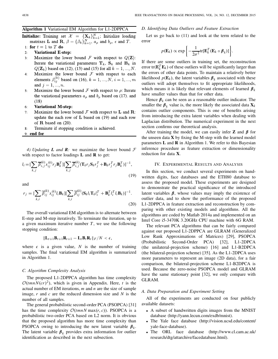
Fig. 1. Digit 5 images with added noises.
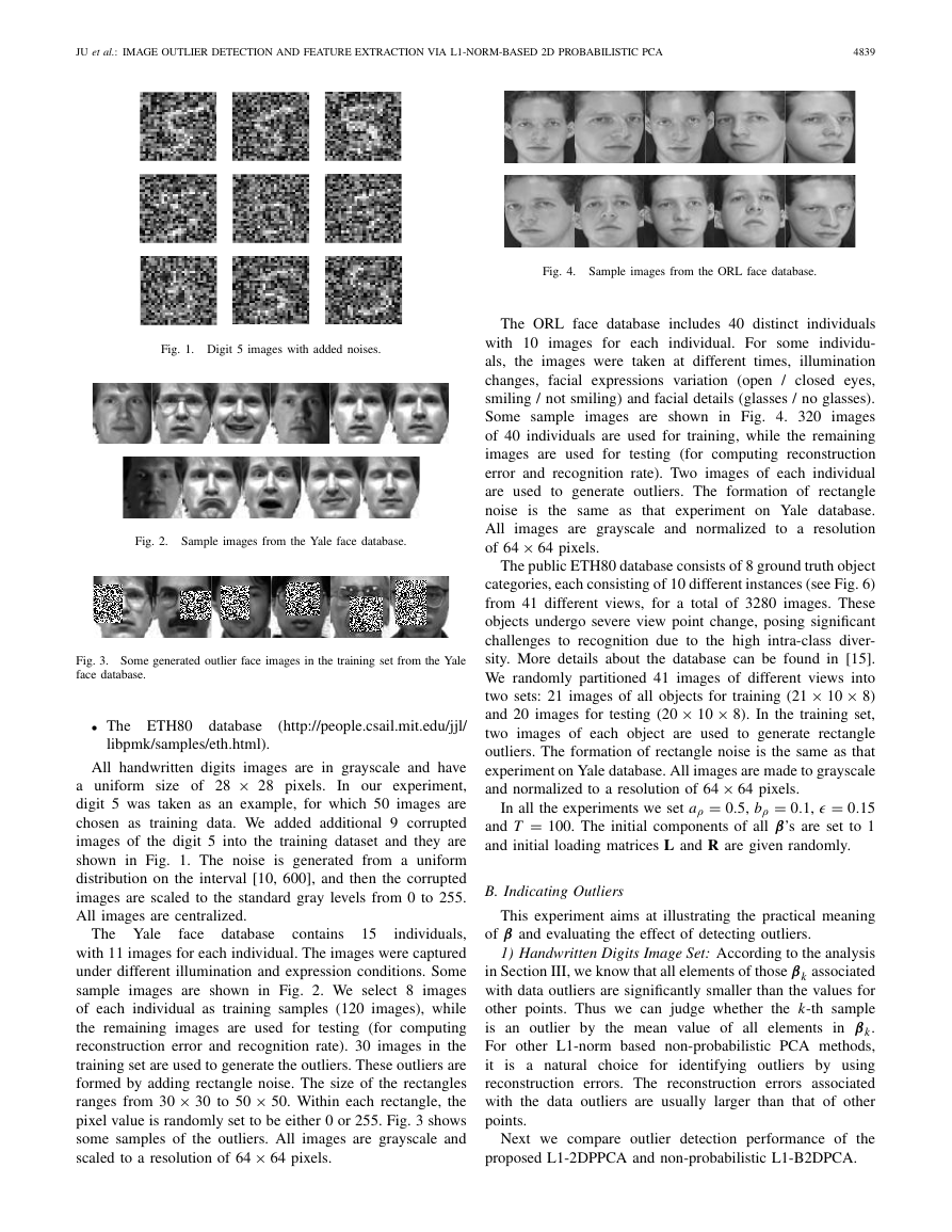
Fig. 2. Sample images from the Yale face database.
Fig. 3. Some generated outlier face images in the training set from the Yale
face database.
• The ETH80
database
libpmk/samples/eth.html).
(http://people.csail.mit.edu/jjl/
All handwritten digits images are in grayscale and have
a uniform size of 28 × 28 pixels.
In our experiment,
digit 5 was taken as an example, for which 50 images are
chosen as training data. We added additional 9 corrupted
images of the digit 5 into the training dataset and they are
shown in Fig. 1. The noise is generated from a uniform
distribution on the interval [10, 600], and then the corrupted
images are scaled to the standard gray levels from 0 to 255.
All images are centralized.
face
contains
15
database
The Yale
individuals,
with 11 images for each individual. The images were captured
under different illumination and expression conditions. Some
sample images are shown in Fig. 2. We select 8 images
of each individual as training samples (120 images), while
the remaining images are used for testing (for computing
reconstruction error and recognition rate). 30 images in the
training set are used to generate the outliers. These outliers are
formed by adding rectangle noise. The size of the rectangles
ranges from 30 × 30 to 50 × 50. Within each rectangle, the
pixel value is randomly set to be either 0 or 255. Fig. 3 shows
some samples of the outliers. All images are grayscale and
scaled to a resolution of 64 × 64 pixels.
Fig. 4. Sample images from the ORL face database.
The ORL face database includes 40 distinct individuals
with 10 images for each individual. For some individu-
als, the images were taken at different times, illumination
changes, facial expressions variation (open / closed eyes,
smiling / not smiling) and facial details (glasses / no glasses).
Some sample images are shown in Fig. 4. 320 images
of 40 individuals are used for training, while the remaining
images are used for testing (for computing reconstruction
error and recognition rate). Two images of each individual
are used to generate outliers. The formation of rectangle
noise is the same as that experiment on Yale database.
All
images are grayscale and normalized to a resolution
of 64 × 64 pixels.
The public ETH80 database consists of 8 ground truth object
categories, each consisting of 10 different instances (see Fig. 6)
from 41 different views, for a total of 3280 images. These
objects undergo severe view point change, posing significant
challenges to recognition due to the high intra-class diver-
sity. More details about the database can be found in [15].
We randomly partitioned 41 images of different views into
two sets: 21 images of all objects for training (21 × 10 × 8)
and 20 images for testing (20 × 10 × 8). In the training set,
two images of each object are used to generate rectangle
outliers. The formation of rectangle noise is the same as that
experiment on Yale database. All images are made to grayscale
and normalized to a resolution of 64 × 64 pixels.
In all the experiments we set aρ = 0.5, bρ = 0.1, � = 0.15
and T = 100. The initial components of all β’s are set to 1
and initial loading matrices L and R are given randomly.
B. Indicating Outliers
This experiment aims at illustrating the practical meaning
of β and evaluating the effect of detecting outliers.
1) Handwritten Digits Image Set: According to the analysis
in Section III, we know that all elements of those βk associated
with data outliers are significantly smaller than the values for
other points. Thus we can judge whether the k-th sample
is an outlier by the mean value of all elements in βk.
For other L1-norm based non-probabilistic PCA methods,
it
identifying outliers by using
reconstruction errors. The reconstruction errors associated
with the data outliers are usually larger than that of other
points.
is a natural choice for
Next we compare outlier detection performance of the
proposed L1-2DPPCA and non-probabilistic L1-B2DPCA.
�
4840
IEEE TRANSACTIONS ON IMAGE PROCESSING, VOL. 24, NO. 12, DECEMBER 2015
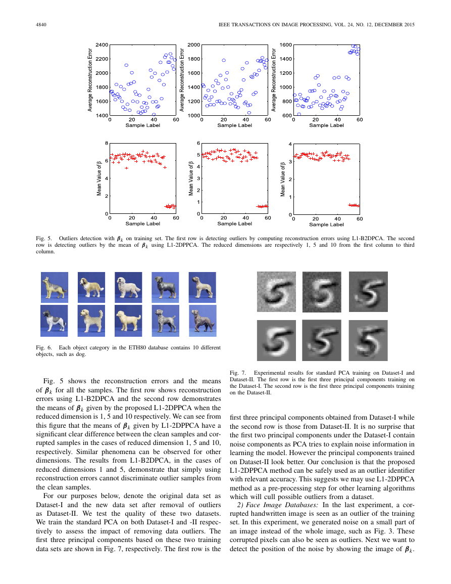
Fig. 5. Outliers detection with βk on training set. The first row is detecting outliers by computing reconstruction errors using L1-B2DPCA. The second
row is detecting outliers by the mean of βk using L1-2DPPCA. The reduced dimensions are respectively 1, 5 and 10 from the first column to third
column.
Fig. 6. Each object category in the ETH80 database contains 10 different
objects, such as dog.
Fig. 5 shows the reconstruction errors and the means
of βk for all the samples. The first row shows reconstruction
errors using L1-B2DPCA and the second row demonstrates
the means of βk given by the proposed L1-2DPPCA when the
reduced dimension is 1, 5 and 10 respectively. We can see from
this figure that the means of βk given by L1-2DPPCA have a
significant clear difference between the clean samples and cor-
rupted samples in the cases of reduced dimension 1, 5 and 10,
respectively. Similar phenomena can be observed for other
dimensions. The results from L1-B2DPCA, in the cases of
reduced dimensions 1 and 5, demonstrate that simply using
reconstruction errors cannot discriminate outlier samples from
the clean samples.
For our purposes below, denote the original data set as
Dataset-I and the new data set after removal of outliers
as Dataset-II. We test
the quality of these two datasets.
We train the standard PCA on both Dataset-I and -II respec-
tively to assess the impact of removing data outliers. The
first three principal components based on these two training
data sets are shown in Fig. 7, respectively. The first row is the
Fig. 7.
Experimental results for standard PCA training on Dataset-I and
Dataset-II. The first row is the first three principal components training on
the Dataset-I. The second row is the first three principal components training
on the Dataset-II.
first three principal components obtained from Dataset-I while
the second row is those from Dataset-II. It is no surprise that
the first two principal components under the Dataset-I contain
noise components as PCA tries to explain noise information in
learning the model. However the principal components trained
on Dataset-II look better. Our conclusion is that the proposed
L1-2DPPCA method can be safely used as an outlier identifier
with relevant accuracy. This suggests we may use L1-2DPPCA
method as a pre-processing step for other learning algorithms
which will cull possible outliers from a dataset.
2) Face Image Databases: In the last experiment, a cor-
rupted handwritten image is seen as an outlier of the training
set. In this experiment, we generated noise on a small part of
an image instead of the whole image, such as Fig. 3. These
corrupted pixels can also be seen as outliers. Next we want to
detect the position of the noise by showing the image of βk.
�
JU et al.: IMAGE OUTLIER DETECTION AND FEATURE EXTRACTION VIA L1-NORM-BASED 2D PROBABILISTIC PCA
4841
Fig. 8. The results of outlier detection with βk on face images. (a) Shows
some generated outlier face images from the Yale face database in the first row.
The second row is the images of βk associated with the first row face images.
(b) Shows some generated outlier face images from the ORL face database
in the first row. The second row is the images of βk associated with the last
row face images.
We tested this method on the Yale and ORL face databases
and the data preparation is given in Section IV.A.
Fig. 8 shows the results of outlier detection with βk. The
first and third rows show some training samples of outlier
face images from the Yale face database and ORL face
database, respectively. The second row shows the images of βk
associated with face images on the first row. The fourth row
shows the images of βk associated with the face images on the
third row. It can be seen that each of all βk images contains
a black block revealing the noise part in the corresponding
outlier face image.
C. Reconstruction Error
In this section, we test reconstruction errors of the models
based on two face datasets (Yale and ORL). As illustrated
in data preparation in Section IV.A,
these two training
sets
include 25% outlier samples. Once the projection
matrices L and R have been trained by using a training dataset,
we can compute the reconstruction errors for any test sample
set. The reconstruction error is computed with respect to the
, where X is the
recovered test sample set and X is the ground-truth test sample
ground truth, which is defined as
X− XF
N
set. N is the number of test samples. The involved algorithms
include GLRAM, L1-B2DPCA, the proposed L1-2DPPCA,
which are 2D feature extraction algorithms, and L1-PPCA,
which is a 1D feature extraction algorithm based on L1-norm.
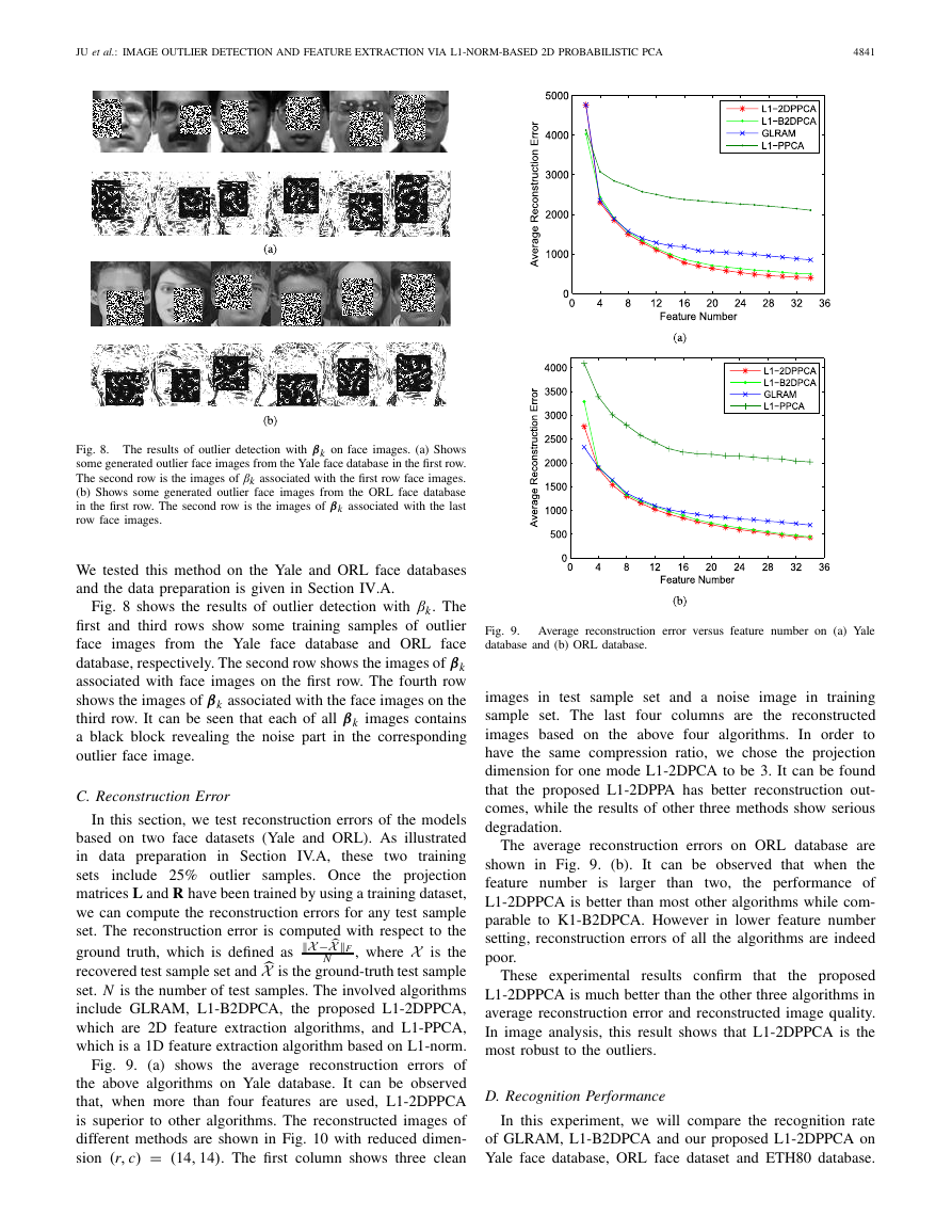
Fig. 9. (a) shows the average reconstruction errors of
the above algorithms on Yale database. It can be observed
that, when more than four features are used, L1-2DPPCA
is superior to other algorithms. The reconstructed images of
different methods are shown in Fig. 10 with reduced dimen-
sion (r, c) = (14, 14). The first column shows three clean
Fig. 9.
database and (b) ORL database.
Average reconstruction error versus feature number on (a) Yale
images in test sample set and a noise image in training
sample set. The last four columns are the reconstructed
images based on the above four algorithms. In order to
have the same compression ratio, we chose the projection
dimension for one mode L1-2DPCA to be 3. It can be found
that the proposed L1-2DPPA has better reconstruction out-
comes, while the results of other three methods show serious
degradation.
The average reconstruction errors on ORL database are
shown in Fig. 9. (b). It can be observed that when the
feature number
the performance of
L1-2DPPCA is better than most other algorithms while com-
parable to K1-B2DPCA. However in lower feature number
setting, reconstruction errors of all the algorithms are indeed
poor.
than two,
is larger
These experimental
results confirm that
the proposed
L1-2DPPCA is much better than the other three algorithms in
average reconstruction error and reconstructed image quality.
In image analysis, this result shows that L1-2DPPCA is the
most robust to the outliers.
D. Recognition Performance
In this experiment, we will compare the recognition rate
of GLRAM, L1-B2DPCA and our proposed L1-2DPPCA on
Yale face database, ORL face dataset and ETH80 database.
�


 2023年江西萍乡中考道德与法治真题及答案.doc
 2012年重庆南川中考生物真题及答案.doc
 2013年江西师范大学地理学综合及文艺理论基础考研真题.doc
 2020年四川甘孜小升初语文真题及答案I卷.doc
 2020年注册岩土工程师专业基础考试真题及答案.doc
 2023-2024学年福建省厦门市九年级上学期数学月考试题及答案.doc
 2021-2022学年辽宁省沈阳市大东区九年级上学期语文期末试题及答案.doc
 2022-2023学年北京东城区初三第一学期物理期末试卷及答案.doc
 2018上半年江西教师资格初中地理学科知识与教学能力真题及答案.doc
 2012年河北国家公务员申论考试真题及答案-省级.doc
 2020-2021学年江苏省扬州市江都区邵樊片九年级上学期数学第一次质量检测试题及答案.doc
 2022下半年黑龙江教师资格证中学综合素质真题及答案.doc