EdgeConnect: Generative Image Inpainting with Adversarial Edge Learning
Kamyar Nazeri, Eric Ng, Tony Joseph, Faisal Qureshi, Mehran Ebrahimi
Faculty of Science, University of Ontario Institute of Technology, Canada
{kamyar.nazeri, eric.ng, tony.joseph, faisal.qureshi, mehran.ebrahimi}@uoit.ca
9
1
0
2
n
a
J
1
]
V
C
.
s
c
[
1
v
2
1
2
0
0
.
1
0
9
1
:
v
i
X
r
a
Abstract
Over the last few years, deep learning techniques have
yielded significant improvements in image inpainting. How-
ever, many of these techniques fail to reconstruct reason-
able structures as they are commonly over-smoothed and/or
blurry. This paper develops a new approach for image in-
painting that does a better job of reproducing filled regions
exhibiting fine details. We propose a two-stage adversarial
model EdgeConnect that comprises of an edge generator
followed by an image completion network. The edge gen-
erator hallucinates edges of the missing region (both reg-
ular and irregular) of the image, and the image comple-
tion network fills in the missing regions using hallucinated
edges as a priori. We evaluate our model end-to-end over
the publicly available datasets CelebA, Places2, and Paris
StreetView, and show that it outperforms current state-of-
the-art techniques quantitatively and qualitatively.
1. Introduction
Image inpainting, or image completion, involves filling
in missing regions of an image. It is an important step in
many image editing tasks. It can, for example, be used to
fill in the holes left after removing unwanted objects from an
image. Humans have an uncanny ability to zero in on visual
inconsistencies. Consequently, the filled regions must be
perceptually plausible. Among other things, the lack of fine
structure in the filled region is a giveaway that something is
amiss, especially when the rest of the image contain sharp
details. The work presented in this paper is motivated by our
observation that many existing image inpainting techniques
generate over-smoothed and/or blurry regions, failing to re-
produce fine details.
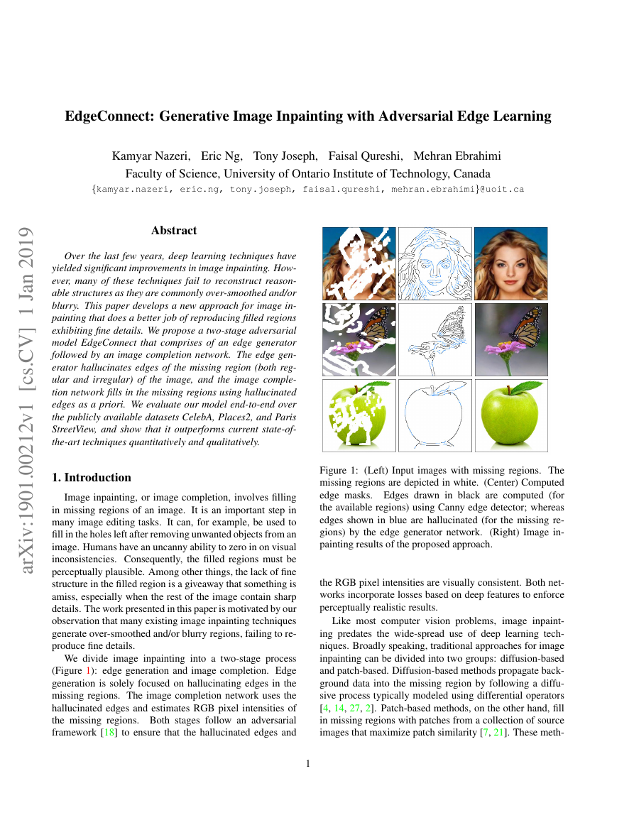
We divide image inpainting into a two-stage process
(Figure 1): edge generation and image completion. Edge
generation is solely focused on hallucinating edges in the
missing regions. The image completion network uses the
hallucinated edges and estimates RGB pixel intensities of
the missing regions. Both stages follow an adversarial
framework [18] to ensure that the hallucinated edges and
Figure 1: (Left) Input images with missing regions. The
missing regions are depicted in white. (Center) Computed
edge masks. Edges drawn in black are computed (for
the available regions) using Canny edge detector; whereas
edges shown in blue are hallucinated (for the missing re-
gions) by the edge generator network.
(Right) Image in-
painting results of the proposed approach.
the RGB pixel intensities are visually consistent. Both net-
works incorporate losses based on deep features to enforce
perceptually realistic results.
Like most computer vision problems, image inpaint-
ing predates the wide-spread use of deep learning tech-
niques. Broadly speaking, traditional approaches for image
inpainting can be divided into two groups: diffusion-based
and patch-based. Diffusion-based methods propagate back-
ground data into the missing region by following a diffu-
sive process typically modeled using differential operators
[4, 14, 27, 2]. Patch-based methods, on the other hand, fill
in missing regions with patches from a collection of source
images that maximize patch similarity [7, 21]. These meth-
1
�
ods, however, do a poor job of reconstructing complex de-
tails that may be local to the missing region.
More recently deep learning approaches have found re-
markable success at the task of image inpainting. These
schemes fill the missing pixels using learned data distribu-
tion. They are able to generate coherent structures in the
missing regions, a feat that was nearly impossible for tradi-
tional techniques. While these approaches are able to gen-
erate missing regions with meaningful structures, the gen-
erated regions are often blurry or suffer from artifacts, sug-
gesting that these methods struggle to reconstruct high fre-
quency information accurately.
Then, how does one force an image inpainting network
to generate fine details? Since image structure is well-
represented in its edge mask, we show that it is possible to
generate superior results by conditioning an image inpaint-
ing network on edges in the missing regions. Clearly, we
do not have access to edges in the missing regions. Rather,
we train an edge generator that hallucinates edges in these
areas. Our approach of “lines first, color next” is partly in-
spired by our understanding of how artists work [13]. “In
line drawing, the lines not only delineate and define spaces
and shapes; they also play a vital role in the composition”,
says Betty Edwards, highlights the importance of sketches
from an artistic viewpoint [12]. Edge recovery, we sup-
pose, is an easier task than image completion. Our proposed
model essentially decouples the recovery of high and low-
frequency information of the inpainted region.
We evaluate our proposed model on standard datasets
CelebA [30], Places2 [56], and Paris StreetView [8]. We
compare the performance of our model against current
state-of-the-art schemes. Furthermore, we provide results
of experiments carried out to study the effects of edge in-
formation on the image inpainting task. Our paper makes
the following contributions:
• An edge generator capable of hallucinating edges in
missing regions given edges and grayscale pixel inten-
sities of the rest of the image.
• An image completion network that combines edges in
the missing regions with color and texture information
of the rest of the image to fill the missing regions.
• An end-to-end trainable network that combines edge
generation and image completion to fill in missing re-
gions exhibiting fine details.
We show that our model can be used in some common im-
age editing applications, such as object removal and scene
generation. Our source code is available at:
https://github.com/knazeri/edge-connect
2. Related Work
Diffusion-based methods propagate neighboring infor-
mation into the missing regions [4, 2].
[14] adapted the
Mumford-Shah segmentation model for image inpainting
2
by introducing Euler’s Elastica. However, reconstruc-
tion is restricted to locally available information for these
diffusion-based methods, and these methods fail to recover
meaningful structures in the missing regions. These meth-
ods also cannot adequately deal with large missing regions.
Patch-based methods fill in missing regions (i.e., targets)
by copying information from similar regions (i.e., sources)
of the same image (or a collection of images). Source re-
gions are often blended into the target regions to minimize
discontinuities [7, 21]. These methods are computation-
ally expensive since similarity scores must be computed for
every target-source pair. PatchMatch [3] addressed this is-
sue by using a fast nearest neighbor field algorithm. These
methods, however, assume that the texture of the inpainted
region can be found elsewhere in the image. This assump-
tion does not always hold. Consequently, these methods
excel at recovering highly patterned regions such as back-
ground completion but struggle at reconstructing patterns
that are locally unique.
One of the first deep learning methods designed for
image inpainting is context encoder [38], which uses an
encoder-decoder architecture. The encoder maps an image
with missing regions to a low-dimensional feature space,
which the decoder uses to construct the output image. How-
ever, the recovered regions of the output image often con-
tain visual artifacts and exhibit blurriness due to the in-
formation bottleneck in the channel-wise fully connected
layer. This was addressed by Iizuka et al. [22] by reduc-
ing the number of downsampling layers, and replacing the
channel-wise fully connected layer with a series of dilated
convolution layers [51]. The reduction of downsampling
layers are compensated by using varying dilation factors.
However, training time was increased significantly1 due to
extremely sparse filters created using large dilation factors.
Yang et al. [49] uses a pre-trained VGG network [42] to
improve the output of the context-encoder, by minimizing
the feature difference of image background. This approach
requires solving a multi-scale optimization problem itera-
tively, which noticeably increases computational cost dur-
ing inference time. Liu et al. [28] introduced “partial convo-
lution” for image inpainting, where convolution weights are
normalized by the mask area of the window that the convo-
lution filter currently resides over. This effectively prevents
the convolution filters from capturing too many zeros when
they traverse over the incomplete region.
Recently, several methods were introduced by providing
additional information prior to inpainting. Yeh et al. [50]
trains a GAN for image inpainting with uncorrupted data.
During inference, back-propagation is employed for 1, 500
iterations to find the representation of the corrupted image
on a uniform noise distribution. However, the model is slow
during inference since back-propagation must be performed
1Model by [22] required two months of training over four GPUs.
�
for every image it attempts to recover. Dolhansky and Fer-
rer [9] demonstrate the importance of exemplar information
for inpainting. Their method is able to achieve both sharp
and realistic inpainting results. Their method, however, is
geared towards filling in missing eye regions in frontal hu-
man face images. It is highly specialized and does not gen-
eralize well. Contextual Attention [53] takes a two-step ap-
proach to the problem of image inpainting. First, it produces
a coarse estimate of the missing region. Next, a refinement
network sharpens the result using an attention mechanism
by searching for a collection of background patches with
the highest similarity to the coarse estimate. [43] takes a
similar approach and introduces a “patch-swap” layer which
replaces each patch inside the missing region with the most
similar patch on the boundary. These schemes suffer from
two limitations: 1) the refinement network assumes that the
coarse estimate is reasonably accurate, and 2) these meth-
ods cannot handle missing regions with arbitrary shapes.
Free-form inpainting method proposed in [52] is perhaps
closest in spirit to our scheme. It uses hand-drawn sketches
to guide the inpainting process. Our method does away with
hand-drawn sketches and instead learns to hallucinate edges
in the missing regions.
2.1. Image-to-Edges vs. Edges-to-Image
The inpainting technique proposed in this paper sub-
sumes two disparate computer vision problems: Image-to-
Edges and Edges-to-Image. There is a large body of liter-
ature that addresses “Image-to-Edges” problems [5, 10, 26,
29]. Canny edge detector, an early scheme for constructing
edge maps, for example, is roughly 30 years old [6]. Doll´ar
and Zitnikc [11] use structured learning [35] on random
decision forests to predict local edge masks. Holistically-
nested Edge Detection (HED) [48] is a fully convolutional
network that learns edge information based on its impor-
tance as a feature of the overall image.
In our work, we
train on edge maps computed using Canny edge detector.
We explain this in detail in Section 4.1 and Section 5.3.
Traditional “Edges-to-Image” methods typically follow
a bag-of-words approach, where image content is con-
structed through a pre-defined set of keywords. These
methods, however, are unable to accurately construct fine-
grained details especially near object boundaries. Scribbler
[41] is a learning-based model where images are generated
using line sketches as the input. The results of their work
possess an art-like quality, where color distribution of the
generated result is guided by the use of color in the input
sketch. Isola et al. [23] proposed a conditional GAN frame-
work [33], called pix2pix, for image-to-image translation
problems. This scheme can use available edge information
as a priori. CycleGAN [57] extends this framework and
finds a reverse mapping back to the original data distribu-
tion. This approach yields superior results since the aim is
to learn the inverse of the forward mapping.
3. EdgeConnect
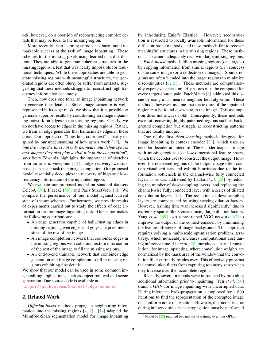
We propose an image inpainting network that consists of
two stages: 1) edge generator, and 2) image completion net-
work (Figure 2). Both stages follow an adversarial model
[18], i.e. each stage consists of a generator/discriminator
pair. Let G1 and D1 be the generator and discriminator for
the edge generator, and G2 and D2 be the generator and dis-
criminator for the image completion network, respectively.
To simplify notation, we will use these symbols also to rep-
resent the function mappings of their respective networks.
Our generators follow an architecture similar to the
method proposed by Johnson et al. [24], which has achieved
impressive results for style transfer, super-resolution [40,
17], and image-to-image translation [57]. Specifically, the
generators consist of encoders that down-sample twice, fol-
lowed by eight residual blocks [19] and decoders that up-
sample images back to the original size. Dilated convolu-
tions with a dilation factor of two are used instead of regular
convolutions in the residual layers, resulting in a receptive
field of 205 at the final residual block. For discriminators,
we use a 70×70 PatchGAN [23, 57] architecture, which de-
termines whether or not overlapping image patches of size
70 × 70 are real. We use instance normalization [45] across
all layers of the network2.
3.1. Edge Generator
Let Igt be ground truth images. Their edge map and
grayscale counterpart will be denoted by Cgt and Igray,
respectively.
In the edge generator, we use the masked
grayscale image ˜Igray = Igray (1 − M) as the input,
its edge map ˜Cgt = Cgt (1− M), and image mask M as
a pre-condition (1 for the missing region, 0 for background).
Here, denotes the Hadamard product. The generator pre-
dicts the edge map for the masked region
˜Igray, ˜Cgt, M
Cpred = G1
.
(1)
We use Cgt and Cpred conditioned on Igray as inputs of
the discriminator that predicts whether or not an edge map
is real. The network is trained with an objective comprised
of an adversarial loss and feature-matching loss [46]
min
G1
max
D1
G1
LG1 = min
(Ladv,1) + λF MLF M
(2)
where λadv,1 and λF M are regularization parameters. The
adversarial loss is defined as
λadv,1 max
D1
Ladv,1 = E(Cgt,Igray) [log D1(Cgt, Igray)]
+ EIgray log [1 − D1(Cpred, Igray)] .
(3)
2The details of our architecture are in appendix A
3
�
Figure 2: Summary of our proposed method. Incomplete grayscale image and edge map, and mask are the inputs of G1 to
predict the full edge map. Predicted edge map and incomplete color image are passed to G2 to perform the inpainting task.
The feature-matching loss LF M compares the activation
maps in the intermediate layers of the discriminator. This
stabilizes the training process by forcing the generator to
produce results with representations that are similar to real
images. This is similar to perceptual loss [24, 16, 15],
where activation maps are compared with those from the
pre-trained VGG network. However, since the VGG net-
work is not trained to produce edge information, it fails to
capture the result that we seek in the initial stage. The fea-
ture matching loss LF M is defined as
LF M = E
1 (Cgt) − D(i)
1 (Cpred)
, (4)
L
i=1
D(i)
1
Ni
1
where L is the final convolution layer of the discriminator,
Ni is the number of elements in the i’th activation layer,
and D(i)
is the activation in the i’th layer of the discrim-
1
inator. Spectral normalization (SN) [34] further stabilizes
training by scaling down weight matrices by their respec-
tive largest singular values, effectively restricting the Lip-
schitz constant of the network to one. Although this was
originally proposed to be used only on the discriminator, re-
cent works [54, 36] suggest that generator can also benefit
from SN by suppressing sudden changes of parameter and
gradient values. Therefore, we apply SN to both generator
and discriminator. Spectral normalization was chosen over
Wasserstein GAN (WGAN), [1] as we found that WGAN
was several times slower in our early tests. Note that only
Ladv,1 is maximized over D1 since D1 is used to retrieve
activation maps for LF M . For our experiments, we choose
λadv,1 = 1 and λF M = 10.
3.2. Image Completion Network
The image completion network uses the incomplete
color image ˜Igt = Igt (1 − M) as input, conditioned
using a composite edge map Ccomp. The composite edge
map is constructed by combining the background region
of ground truth edges with generated edges in the cor-
rupted region from the previous stage, i.e. Ccomp = Cgt
(1 − M) + Cpred M. The network returns a color im-
4
age Ipred, with missing regions filled in, that has the same
resolution as the input image:
˜Igt, Ccomp
Ipred = G2
.
(5)
i
This is trained over a joint loss that consists of an 1 loss,
adversarial loss, perceptual loss, and style loss. To ensure
proper scaling, the 1 loss is normalized by the mask size.
The adversarial loss is defined similar to Eq. 3, as
Ladv,2 = E(Igt,Ccomp) [log D2(Igt, Ccomp)]
+ ECcomp log [1 − D2(Ipred, Ccomp)] .
(6)
We include the two losses proposed in [16, 24] commonly
known as perceptual loss Lperc and style loss Lstyle. As
the name suggests, Lperc penalizes results that are not per-
ceptually similar to labels by defining a distance measure
between activation maps of a pre-trained network. Percep-
tual loss is defined as
Lperc = E
φi(Igt) − φi(Ipred)1
1
Ni
(7)
where φi is the activation map of the i’th layer of a pre-
trained network. For our work, φi corresponds to activation
maps from layers relu1 1, relu2 1, relu3 1, relu4 1
and relu5 1 of the VGG-19 network pre-trained on the Im-
ageNet dataset [39]. These activation maps are also used to
compute style loss which measures the differences between
covariances of the activation maps. Given feature maps of
sizes Cj × Hj × Wj, style loss is computed by
j (˜Igt)1
Lstyle = Ej
(8)
j is a Cj × Cj Gram matrix constructed from ac-
where Gφ
tivation maps φj. We choose to use style loss as it was
shown by Sajjadi et al. [40] to be an effective tool to com-
bat “checkerboard” artifacts caused by transpose convolu-
tion layers [37]. Our overall loss function is
LG2 = λ1L1 + λadv,2Ladv,2 + λpLperc + λsLstyle. (9)
j (˜Ipred) − Gφ
Gφ
Dilated Conv + Residual BlocksMask + Edge + GrayscaleEdge Map+H x WH x WH/2 x W/2H/2 x W/2H/4 x W/4Feature Matching ( LFM )Real/Fake ( Ladv,1 )Dilated Conv + Residual BlocksH x WH x WH/2 x W/2H/2 x W/2H/4 x W/4InputOutputReconstruction ( L1)Perceptual ( Lperc )Style ( Lstyle ) Perceptual ( Lperc )Style ( Lstyle ) Reconstruction ( L1)Real/Fake ( Ladv,2 )G1D1D2G2�
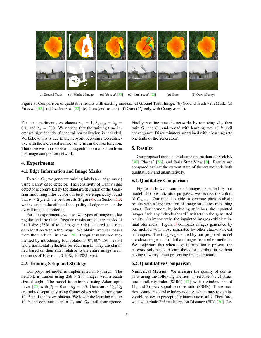
(a) Ground Truth
(b) Masked Image
(c) Yu et al. [53]
(d) Iizuka et al. [22]
(e) Ours
(f) Ours (Canny)
Figure 3: Comparison of qualitative results with existing models. (a) Ground Truth Image. (b) Ground Truth with Mask. (c)
Yu et al. [53]. (d) Iizuka et al. [22]. (e) Ours (end-to-end). (f) Ours (G2 only with Canny σ = 2).
For our experiments, we choose λ1 = 1, λadv,2 = λp =
0.1, and λs = 250. We noticed that the training time in-
creases significantly if spectral normalization is included.
We believe this is due to the network becoming too restric-
tive with the increased number of terms in the loss function.
Therefore we choose to exclude spectral normalization from
the image completion network.
4. Experiments
4.1. Edge Information and Image Masks
To train G1, we generate training labels (i.e. edge maps)
using Canny edge detector. The sensitivity of Canny edge
detector is controlled by the standard deviation of the Gaus-
sian smoothing filter σ. For our tests, we empirically found
that σ ≈ 2 yields the best results (Figure 6). In Section 5.3,
we investigate the effect of the quality of edge maps on the
overall image completion.
For our experiments, we use two types of image masks:
regular and irregular. Regular masks are square masks of
fixed size (25% of total image pixels) centered at a ran-
dom location within the image. We obtain irregular masks
from the work of Liu et al. [28]. Irregular masks are aug-
mented by introducing four rotations (0◦, 90◦, 180◦, 270◦)
and a horizontal reflection for each mask. They are classi-
fied based on their sizes relative to the entire image in in-
crements of 10% (e.g., 0-10%, 10-20%, etc.).
4.2. Training Setup and Strategy
Our proposed model is implemented in PyTorch. The
network is trained using 256 × 256 images with a batch
size of eight. The model is optimized using Adam opti-
mizer [25] with β1 = 0 and β2 = 0.9. Generators G1, G2
are trained separately using Canny edges with learning rate
10−4 until the losses plateau. We lower the learning rate to
10−5 and continue to train G1 and G2 until convergence.
Finally, we fine-tune the networks by removing D1, then
train G1 and G2 end-to-end with learning rate 10−6 until
convergence. Discriminators are trained with a learning rate
one tenth of the generators’.
5. Results
Our proposed model is evaluated on the datasets CelebA
[30], Places2 [56], and Paris StreetView [8]. Results are
compared against the current state-of-the-art methods both
qualitatively and quantitatively.
5.1. Qualitative Comparison
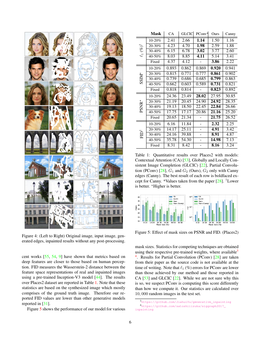
Figure 4 shows a sample of images generated by our
model. For visualization purposes, we reverse the colors
of Ccomp. Our model is able to generate photo-realistic
results with a large fraction of image structures remaining
intact. Furthermore, by including style loss, the inpainted
images lack any “checkerboard” artifacts in the generated
results. As importantly, the inpainted images exhibit min-
imal blurriness. Figure 3 compares images generated by
our method with those generated by other state-of-the-art
techniques. The images generated by our proposed model
are closer to ground truth than images from other methods.
We conjecture that when edge information is present, the
network only needs to learn the color distribution, without
having to worry about preserving image structure.
5.2. Quantitative Comparison
Numerical Metrics We measure the quality of our re-
sults using the following metrics: 1) relative 1; 2) struc-
tural similarity index (SSIM) [47], with a window size of
11; and 3) peak signal-to-noise ratio (PSNR). These met-
rics assume pixel-wise independence, which may assign fa-
vorable scores to perceptually inaccurate results. Therefore,
we also include Fr´echet Inception Distance (FID) [20]. Re-
5
�
Mask
CA
10-20% 2.41
20-30% 4.23
30-40% 6.15
40-50% 8.03
4.37
Fixed
10-20% 0.893
20-30% 0.815
30-40% 0.739
40-50% 0.662
0.818
Fixed
10-20% 24.36
20-30% 21.19
30-40% 19.13
40-50% 17.75
20.65
Fixed
10-20% 6.16
20-30% 14.17
30-40% 24.16
40-50% 35.78
8.31
Fixed
†
)
%
(
1
M
I
S
S
R
N
S
P
†
D
I
F
1.14
1.98
3.02
4.11
0.869
0.777
0.685
0.589
GLCIC PConv* Ours
1.50
2.66
2.59
4.70
3.77
6.78
8.85
5.14
3.86
4.12
0.920
0.862
0.861
0.771
0.799
0.686
0.731
0.603
0.823
0.814
27.95
23.49
24.92
20.45
22.84
18.50
21.16
17.17
21.75
21.34
2.32
11.84
4.91
25.11
8.91
39.88
14.98
54.30
8.16
8.42
28.02
24.90
22.45
20.86
-
-
-
-
-
-
-
-
Canny
1.16
1.88
2.60
3.41
2.22
0.941
0.902
0.863
0.821
0.892
30.85
28.35
26.66
25.20
26.52
2.25
3.42
4.87
7.13
3.24
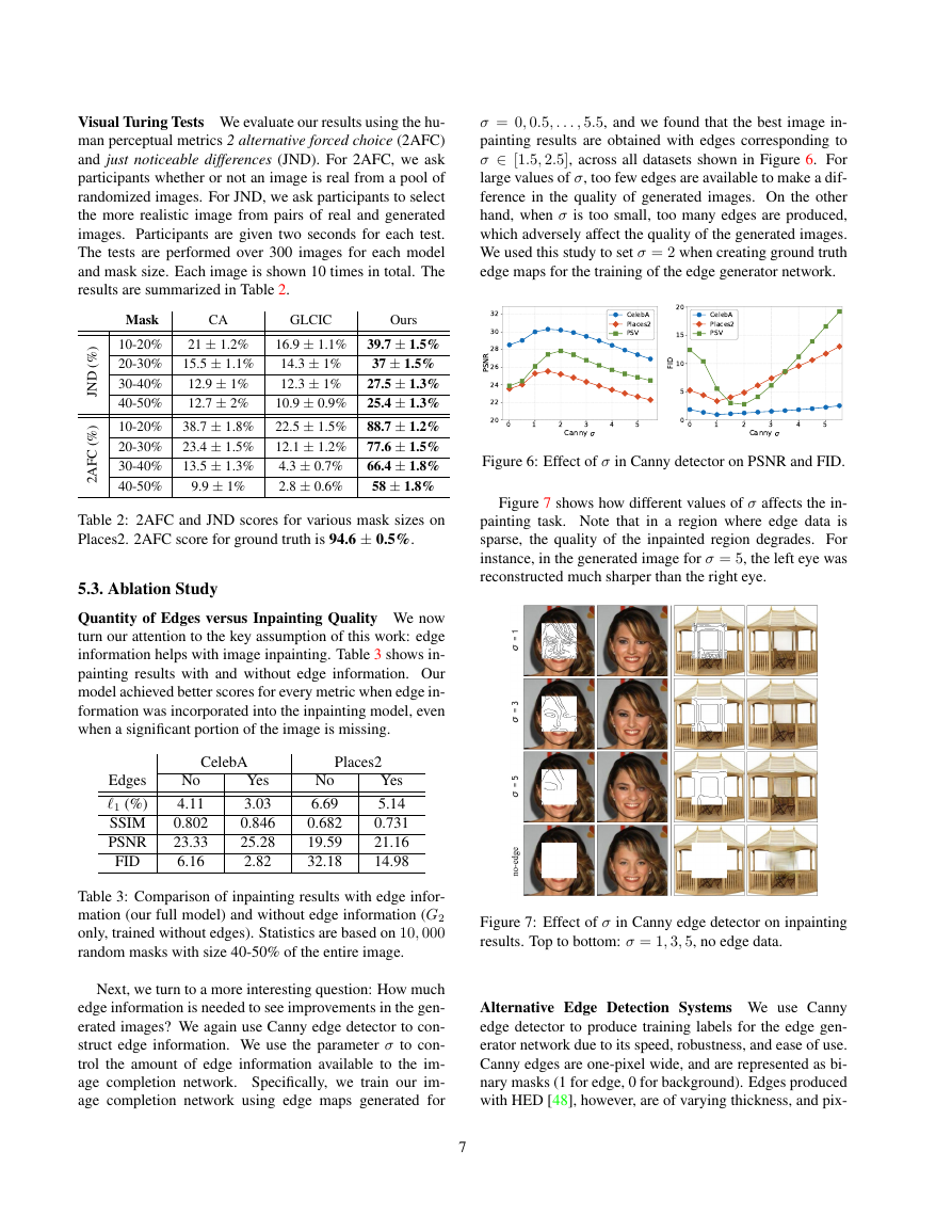
Table 1: Quantitative results over Places2 with models:
Contextual Attention (CA) [53], Globally and Locally Con-
sistent Image Completion (GLCIC) [22], Partial Convolu-
tion (PConv) [28], G1 and G2 (Ours), G2 only with Canny
edges (Canny). The best result of each row is boldfaced ex-
cept for Canny. *Values taken from the paper [28]. †Lower
is better. Higher is better.
Figure 4: (Left to Right) Original image, input image, gen-
erated edges, inpainted results without any post-processing.
cent works [55, 54, 9] have shown that metrics based on
deep features are closer to those based on human percep-
tion. FID measures the Wasserstein-2 distance between the
feature space representations of real and inpainted images
using a pre-trained Inception-V3 model [44]. The results
over Places2 dataset are reported in Table 1. Note that these
statistics are based on the synthesized image which mostly
comprises of the ground truth image. Therefore our re-
ported FID values are lower than other generative models
reported in [31].
Figure 5 shows the performance of our model for various
Figure 5: Effect of mask sizes on PSNR and FID. (Places2)
mask sizes. Statistics for competing techniques are obtained
using their respective pre-trained weights, where available3
4. Results for Partial Convolution (PConv) [28] are taken
from their paper as the source code is not available at the
time of writing. Note that 1 (%) errors for PConv are lower
than those achieved by our method and those reported in
CA [53] and GLCIC [22]. While we are not sure why this
is so, we suspect PConv is computing this score differently
than how we compute it. Our statistics are calculated over
10, 000 random images in the test set.
3https://github.com/JiahuiYu/generative_inpainting
4https://github.com/satoshiiizuka/siggraph2017_
inpainting
6
0-1010-2020-3030-4040-5050-60Mask Size (%)10152025303540PSNRCAGLCICOursOurs (Canny)0-1010-2020-3030-4040-5050-60Mask Size (%)100101102FIDCAGLCICOursOurs (Canny)�
Visual Turing Tests We evaluate our results using the hu-
man perceptual metrics 2 alternative forced choice (2AFC)
and just noticeable differences (JND). For 2AFC, we ask
participants whether or not an image is real from a pool of
randomized images. For JND, we ask participants to select
the more realistic image from pairs of real and generated
images. Participants are given two seconds for each test.
The tests are performed over 300 images for each model
and mask size. Each image is shown 10 times in total. The
results are summarized in Table 2.
σ = 0, 0.5, . . . , 5.5, and we found that the best image in-
painting results are obtained with edges corresponding to
σ ∈ [1.5, 2.5], across all datasets shown in Figure 6. For
large values of σ, too few edges are available to make a dif-
ference in the quality of generated images. On the other
hand, when σ is too small, too many edges are produced,
which adversely affect the quality of the generated images.
We used this study to set σ = 2 when creating ground truth
edge maps for the training of the edge generator network.
CA
GLCIC
Ours
Mask
) 10-20%
%
(
D
N
J
21 ± 1.2%
20-30% 15.5 ± 1.1%
12.9 ± 1%
30-40%
12.7 ± 2%
40-50%
16.9 ± 1.1% 39.7 ± 1.5%
14.3 ± 1%
37 ± 1.5%
12.3 ± 1%
27.5 ± 1.3%
10.9 ± 0.9% 25.4 ± 1.3%
) 10-20% 38.7 ± 1.8% 22.5 ± 1.5% 88.7 ± 1.2%
20-30% 23.4 ± 1.5% 12.1 ± 1.2% 77.6 ± 1.5%
66.4 ± 1.8%
30-40% 13.5 ± 1.3%
9.9 ± 1%
58 ± 1.8%
40-50%
4.3 ± 0.7%
2.8 ± 0.6%
%
(
C
F
A
2
Table 2: 2AFC and JND scores for various mask sizes on
Places2. 2AFC score for ground truth is 94.6 ± 0.5%.
5.3. Ablation Study
Quantity of Edges versus Inpainting Quality We now
turn our attention to the key assumption of this work: edge
information helps with image inpainting. Table 3 shows in-
painting results with and without edge information. Our
model achieved better scores for every metric when edge in-
formation was incorporated into the inpainting model, even
when a significant portion of the image is missing.
Figure 6: Effect of σ in Canny detector on PSNR and FID.
Figure 7 shows how different values of σ affects the in-
painting task. Note that in a region where edge data is
sparse, the quality of the inpainted region degrades. For
instance, in the generated image for σ = 5, the left eye was
reconstructed much sharper than the right eye.
Edges
1 (%)
SSIM
PSNR
FID
No
4.11
0.802
23.33
6.16
Yes
5.14
0.731
21.16
14.98
CelebA
Places2
Yes
3.03
0.846
25.28
2.82
No
6.69
0.682
19.59
32.18
Table 3: Comparison of inpainting results with edge infor-
mation (our full model) and without edge information (G2
only, trained without edges). Statistics are based on 10, 000
random masks with size 40-50% of the entire image.
Next, we turn to a more interesting question: How much
edge information is needed to see improvements in the gen-
erated images? We again use Canny edge detector to con-
struct edge information. We use the parameter σ to con-
trol the amount of edge information available to the im-
age completion network. Specifically, we train our im-
age completion network using edge maps generated for
Figure 7: Effect of σ in Canny edge detector on inpainting
results. Top to bottom: σ = 1, 3, 5, no edge data.
Alternative Edge Detection Systems We use Canny
edge detector to produce training labels for the edge gen-
erator network due to its speed, robustness, and ease of use.
Canny edges are one-pixel wide, and are represented as bi-
nary masks (1 for edge, 0 for background). Edges produced
with HED [48], however, are of varying thickness, and pix-
7
012345Canny 20222426283032PSNRCelebAPlaces2PSV012345Canny 05101520FIDCelebAPlaces2PSV�
els can have intensities ranging between 0 and 1. We no-
ticed that it is possible to create edge maps that look eerily
similar to human sketches by performing element-wise mul-
tiplication on Canny and HED edge maps (Figure 8). We
trained our image completion network using the combined
edge map. However, we did not notice any improvements
in the inpainting results.5
(a)
(d)
Figure 8: (a) Image. (b) Canny. (c) HED. (d) CannyHED.
(b)
(c)
(a)
(b)
(c)
(d)
Figure 10: Edge-map (c) generated using the left-half of (a)
(shown in black) and right-half of (b) (shown in red). Input
is (a) with the right-half removed, producing the output (d).
6. Discussions and Future Work
We proposed EdgeConnect, a new deep learning model
for image inpainting tasks. EdgeConnect comprises of an
edge generator and an image completion network, both fol-
lowing an adversarial model. We demonstrate that edge in-
formation plays an important role in the task of image in-
painting. Our method achieves state-of-the-art results on
standard benchmarks, and is able to deal with images with
multiple, irregularly shaped missing regions.
The trained model can be used as an interactive image
editing tool. We can, for example, manipulate objects in the
edge domain and transform the edge maps back to generate
a new image. This is demonstrated in Figure 10. Here we
have removed the right-half of a given image to be used as
input. The edge maps, however, are provided by a different
image. The generated image seems to share characteristics
of the two images. Figure 11 shows examples where we
attempt to remove unwanted objects from existing images.
We plan to investigate better edge detectors. While effec-
tively delineating the edges is more useful than hundreds of
detailed lines, our edge generating model sometimes fails
to accurately depict the edges in highly textured areas, or
when a large portion of the image is missing (as seen in
Figure 9). We believe our fully convolutional generative
model can be extended to very high-resolution inpainting
applications with an improved edge generating system.
Figure 11: Examples of object removal and image edit-
ing using our EdgeConnect model. (Left) Original image.
(Center) Unwanted object removed with optional edge in-
formation to guide inpainting. (Right) Generated image.
Figure 9: Inpainted results where edge generator fails to
produce relevant edge information.
5Further analysis with HED are available in appendix C.
8
�


 2023年江西萍乡中考道德与法治真题及答案.doc
 2012年重庆南川中考生物真题及答案.doc
 2013年江西师范大学地理学综合及文艺理论基础考研真题.doc
 2020年四川甘孜小升初语文真题及答案I卷.doc
 2020年注册岩土工程师专业基础考试真题及答案.doc
 2023-2024学年福建省厦门市九年级上学期数学月考试题及答案.doc
 2021-2022学年辽宁省沈阳市大东区九年级上学期语文期末试题及答案.doc
 2022-2023学年北京东城区初三第一学期物理期末试卷及答案.doc
 2018上半年江西教师资格初中地理学科知识与教学能力真题及答案.doc
 2012年河北国家公务员申论考试真题及答案-省级.doc
 2020-2021学年江苏省扬州市江都区邵樊片九年级上学期数学第一次质量检测试题及答案.doc
 2022下半年黑龙江教师资格证中学综合素质真题及答案.doc