On Map Matching Vehicle Tracking Data.pdf )

发布时间：2022-06-16 发布人：admin 分类：说明书资料大小：0.54M 资料格式：pdf 举报版权申诉

8cc1d047-2d99-4083-b108-1942db96792b.pdf-第1页.png

第1页 / 共13页

8cc1d047-2d99-4083-b108-1942db96792b.pdf-第2页.png

第2页 / 共13页

8cc1d047-2d99-4083-b108-1942db96792b.pdf-第3页.png

第3页 / 共13页

8cc1d047-2d99-4083-b108-1942db96792b.pdf-第4页.png

第4页 / 共13页

8cc1d047-2d99-4083-b108-1942db96792b.pdf-第5页.png

第5页 / 共13页

8cc1d047-2d99-4083-b108-1942db96792b.pdf-第6页.png

第6页 / 共13页

8cc1d047-2d99-4083-b108-1942db96792b.pdf-第7页.png

第7页 / 共13页

8cc1d047-2d99-4083-b108-1942db96792b.pdf-第8页.png

第8页 / 共13页

文本预览

See discussions, stats, and author profiles for this publication at: https://www.researchgate.net/publication/221310236 On Map-Matching Vehicle Tracking Data. Conference Paper · January 2005 Source: DBLP CITATIONS 228 4 authors, including: READS 97 Sotiris Brakatsoulas Athena-Research and Innovation Center in In… Dieter Pfoser George Mason University 9 PUBLICATIONS 365 CITATIONS 161 PUBLICATIONS 3,190 CITATIONS SEE PROFILE SEE PROFILE Carola Wenk Tulane University 66 PUBLICATIONS 1,136 CITATIONS SEE PROFILE All in-text references underlined in blue are linked to publications on ResearchGate, letting you access and read them immediately. Available from: Dieter Pfoser Retrieved on: 14 May 2016

On Map-Matching Vehicle Tracking Data Sotiris Brakatsoulas1 Dieter Pfoser1 Randall Salas2 Carola Wenk2 1RA Computer Technology Institute Akteou 11 GR-11851 Athens,Greece {sbrakats, pfoser}@cti.gr 2Department of Computer Science University of Texas at San Antonio San Antonio, TX 78249-0667, USA {rsalas, carola}@cs.utsa.edu Abstract Vehicle tracking data is an essential “raw” ma- terial for a broad range of applications such as traﬃc management and control, routing, and navigation. An important issue with this data is its accuracy. The method of sampling vehicular movement using GPS is aﬀected by two error sources and consequently produces inaccurate trajectory data. To become use- ful, the data has to be related to the under- lying road network by means of map match- ing algorithms. We present three such algo- rithms that consider especially the trajectory nature of the data rather than simply the cur- rent position as in the typical map-matching case. An incremental algorithm is proposed that matches consecutive portions of the tra- jectory to the road network, eﬀectively trad- ing accuracy for speed of computation. In contrast, the two global algorithms compare the entire trajectory to candidate paths in the road network. The algorithms are evaluated in terms of (i) their running time and (ii) the quality of their matching result. Two novel quality measures utilizing the Fr´echet distance are introduced and subsequently used in an experimental evaluation to assess the quality of matching real tracking data to a road net- work. 1 Introduction As roads become more and more congested, much re- search is conducted in the area of traﬃc estimation and Permission to copy without fee all or part of this material is granted provided that the copies are not made or distributed for direct commercial advantage, the VLDB copyright notice and the title of the publication and its date appear, and notice is given that copying is by permission of the Very Large Data Base Endowment. To copy otherwise, or to republish, requires a fee and/or special permission from the Endowment. Proceedings of the 31st VLDB Conference, Trondheim, Norway, 2005 prediction systems (TREPS). TREPS use traﬃc mod- els together with sensor data to assess the current and to predict the future traﬃc conditions in the road net- work. Currently, the data component consists of traf- ﬁc counts (quantitative data) obtained by stationary sensors, typically loop detectors, which are deployed throughout the road network. In recent years, a new sensor technology is utilized to complement station- ary sensor networks. Floating car data (FCD) refers to using data generated by one vehicle as a sample to assess the overall traﬃc conditions (“cork swimming in the river”). Typically this data comprises basic ve- hicle telemetry such as speed direction and most im- portantly the position of the vehicle. Recording the position of vehicles in time produces tracking data, of which, in connection with a road network, travel time data (qualitative data) is derived. Having large num- bers of vehicles collecting such data for a given spatial area such as a city (e.g., taxis, public transport, utility vehicles, private vehicles, etc.) will create an accurate picture of the traﬃc condition in time and space [10]. Data management techniques for such FCD collections are presented in [6]. The tracking data is obtained by sampling the po- sitions using typically GPS to produce data that in database terms is commonly referred to as trajecto- ries. Unfortunately, this data is not precise due to the measurement error caused by the limited GPS accu- racy, and the sampling error caused by the sampling rate [14]. A pre-processing step that matches the tra- jectories to the road network is needed. This technique is commonly referred to as map matching. Most map-matching algorithms are tailored towards mapping current positions onto a vector representa- tion of a road network. Onboard systems for vehicle navigation utilize besides continuous positioning also dead reckoning to minimize the positioning error and to produce accurate vehicle positions that can be easily matched to a road map. In the given context, the en- tire trajectory given as a sequence of historic position samples needs to be mapped. The fundamental dif- ference in these two approaches is the error associated with the data. Whereas the data in the former case is 853

mostly aﬀected by the measurement error, the latter case is mostly concerned with the sampling error. We present three map-matching algorithms that map a trajectory onto a road network by matching geometries. The methods diﬀer in the portion of the trajectory they consider for this task. The ﬁrst ap- proach employs an incremental match of the position samples by pursuing a local match of geometries, i.e., matching a portion of the trajectory onto a path in the road network by using a measure composed of distance and angles between the curves. This approach eﬀec- tively trades accuracy for speed of computation. The second approach aims for a global match mapping the entire trajectory to a candidate curve in the road net- work. Two similarity measures are used, the Fr´echet distance and the weak Fr´echet distance, resulting in two diﬀerent map-matching algorithms which guaran- tee to ﬁnd a matching curve with optimal distance to the trajectory. Assessing the quality of the matching result is chal- lenging since for vehicle tracking data typically the “true” path of the vehicle in the road network is not known. Thus, in order to still be able to evaluate the quality of the matching result, a distance measure be- tween the trajectory and the matched path in the road network is needed. We propose two quality measures: (i) the Fr´echet distance and (ii) the average Fr´echet distance. In an experimental evaluation, real track- ing data is used to evaluate the matching results in a practical setting. The speed of computation is as- sessed through analytical cost formulae detailing the running times of the algorithms. The Fr´echet distance for two curves has been pro- posed by Fr´echet [8], and Alt et al. [2] gave an al- gorithm for its computation. Although of practical interest, variations of the Fr´echet distance such as summed or average Fr´echet distance (c.f. Section 5.2) have not yet been considered in the literature. Com- puting the integral Fr´echet distance is an open problem and addressed in this work. Alt et al. [1] give a map- matching algorithm based on the Fr´echet distance. We will sketch this algorithm in Section 4.3. In addition, we propose to utilize the weak Fr´echet distance which results in a map-matching algorithm with a reduced running time while at the same time producing iden- tical matching results for trajectories. Work in the area of map-matching vehicle positions exists towards augmenting GPS positioning with other methods such as dead reckoning to reduce the mea- surement error and to achieve better map-matching results (cf. [15]). Greenfeld [9] introduces a map- matching strategy based on distance and orientation that does not assert any further knowledge about the movement besides the position samples. This algo- rithm serves as the basic strategy for the algorithm introduced in Section 3. Civilis et al. [7] in their work on location update techniques for the tracking of users in location-based services introduce a map-matching algorithm that is based on edge distance and direction similar to [9]. The tracking data itself is obtained by using an active sampling technique based on predicted and measured positions. By controlling the sampling rate, the sampling error can be kept minimal and the map-matching algorithm is presented with an opti- mal dataset. Yin and Wolfson [18] propose an algo- rithm based on a weighted graph representation of the road network in which the weights of each edge rep- resent the distance of the edge to the trajectory. The matched trajectory in the road network is found by us- ing a Dikstra shortest-path algorithm for the weighted graph. This algorithm is based on a measure related to the average Fr´echet distance, however no overall quality guarantee on the matched curve is given. The authors claim that the algorithm produces high qual- ity matches, however details on the data set, such as type and size are missing. Finally, a general introduc- tion to the map-matching problem as addressed in this work can be found in [5]. The outline of this paper is as follows. Section 2 dis- cusses tracking data and introduces the error sources that aﬀect it to derive requirements for map-matching algorithms. Sections 3 and 4 detail the incremental and the global map-matching algorithms, respectively. Section 5 deﬁnes the measures to assess the quality of the map-matching result. Section 6 shows the outcome of the experimental evaluation and, ﬁnally, Section 7 gives conclusions and directions for future research. 2 Motivation and Background The objective of this work is to develop map-matching algorithms for vehicle tracking data that are used as a sensor data source to assess and predict the traﬃc condition in related applications. This section overall describes the properties of the tracking data with a focus on its accuracy to deﬁne requirements for map- matching algorithms. 2.1 Imprecise Trajectory Data The tracking data can be modeled in terms of a tra- jectory, which is obtained by interpolating the position samples. Typically, linear interpolation is used as op- posed to other methods such as polynomial splines. The sampled positions then become the endpoints of line segments of polylines, and the movement of an object is represented by an entire polyline in 3D space [14]. The positioning technology of choice for vehicle tracking is typically GPS. Its associated measurement error in connection with the sampling rate require us to match position samples to the road network. 2.1.1 Measurement Error Two assumptions are generally made about the accu- racy of GPS. First, the error distribution, i.e., the error 854

in each of the three dimensions and the error in time, is assumed to be Gaussian. Second, we can assume that the horizontal error distribution, i.e., the distribution in the x-y plane, is circular [17]. The error in a positional GPS measurement can be described by the probability function following a bi- variate normal distribution [11]. The probability func- tion is composed of two normal distributions in the two respective spatial dimensions. The mean of the distri- bution is the origin of the coordinate system. Fig. 1 visualizes the error distribution. In addition to the mean, the standard deviation, σ, is the characteris- tic parameter stated when referring to GPS accuracy, e.g., 5m GPS accuracy refers to σ. Within the range of ±σ of the mean, in a bivariate normal distribution, 39.35% of the probability is concentrated. Although the GPS error can be substantial in cer- tain situations (shadowed and reﬂected signals), with the use of augmenting the GPS signal (WAAS, EG- NOS) the typical error is in the range of 8m to 2m. The following section discusses the sampling error, which in the case of vehicle tracking data is by two magnitudes larger than the measurement error and consequently has a larger impact on the algorithmic design of a map-matching algorithm. probability y x circular positional error Figure 1: Measurement error for GPS. 2.1.2 Sampling Error The uncertainty of the representation of an object’s movement is aﬀected by the frequency with which po- sition samples are taken, the sampling rate. To il- lustrate the impact of the sampling rate on the im- precision of the interpolated trajectory data, consider sampling the position of a vehicle every 30s, which is a typical sampling rate used in vehicle tracking appli- cations. At a speed of 50km/h, the traveled distance between position samples is as much as 417m! Not measuring the positions in-between two consec- utive position samples, the best we can do is to limit the possibilities of where the moving object could have been. The trajectory can be constrained by what we know about the object’s actual movement. The authors in [14] show that the sampling error between two positions, P1 and P2 in the time interval [t1, t2] and a given maximum speed, vm, for a time tx with t1 < tx < t2 is bound by a lens-shaped proba- bility distribution. 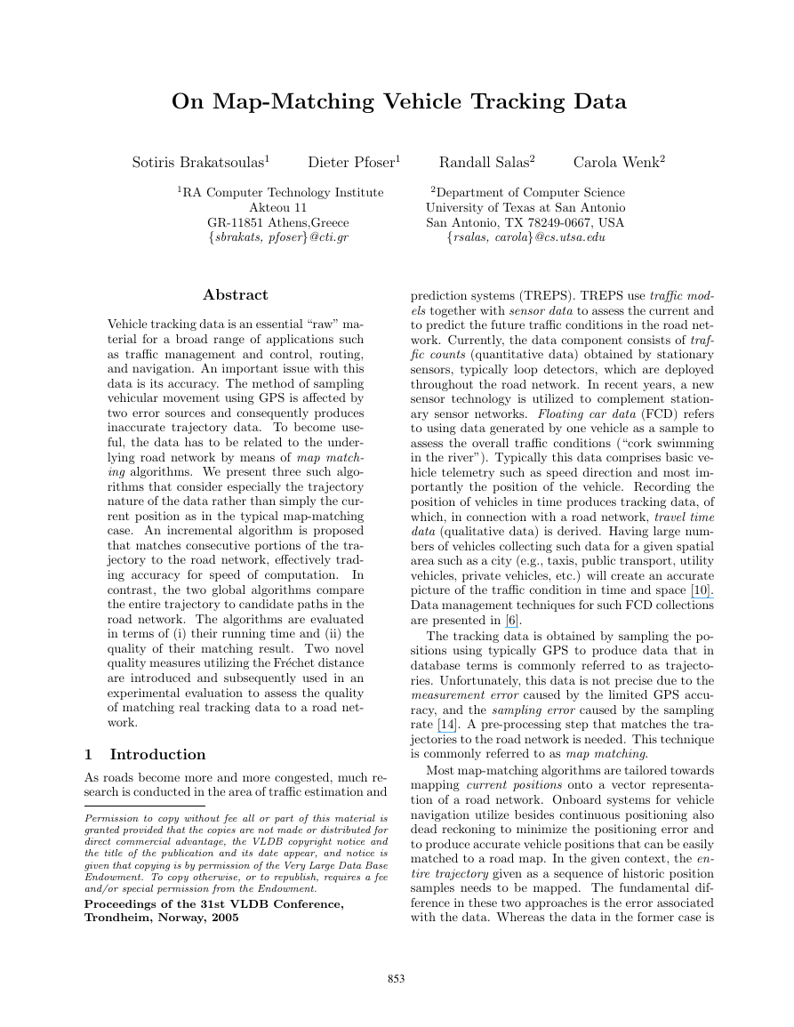Computing the sampling error for various instances of tx shows that a possible trajec- tory between P1 and P2 is overall bound by an error ellipse (cf. Fig. 2). The foci of the ellipse are the sam- pled positions P1 and P2 and the eccentricity 2c is the Euclidean distance between P1 and P2. The length of the semi-major axis, 2a, is the maximum distance the object can travel. If the sampling rate r is given in seconds and the velocity is v km/h then 2a = 5/18 · vr. The “thickness” of the ellipse, 2b, is determined by the equation b2 = a2 − c2 = 25/362 · v2r2 − c2. In simple words, the faster the object travels and the closer its path to that of a linear trajectory, the “thinner” the ellipse. In extreme cases, the ellipse degrades to a line, or even to a point in case the object stopped. 2 2P (x , y , t ) 2 2 2b P (x , y , t ) 1 1 1 1 s max s max s 2c 2a Figure 2: Error ellipse. 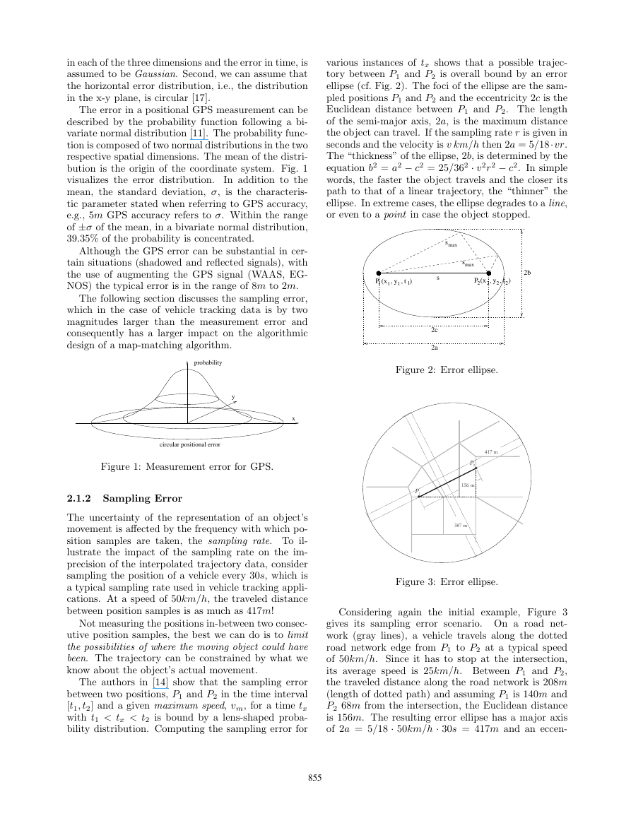417 m P 2 156 m P 1 387 m Figure 3: Error ellipse. Considering again the initial example, Figure 3 gives its sampling error scenario. On a road net- work (gray lines), a vehicle travels along the dotted road network edge from P1 to P2 at a typical speed of 50km/h. Since it has to stop at the intersection, its average speed is 25km/h. Between P1 and P2, the traveled distance along the road network is 208m (length of dotted path) and assuming P1 is 140m and P2 68m from the intersection, the Euclidean distance is 156m. The resulting error ellipse has a major axis of 2a = 5/18 · 50km/h · 30s = 417m and an eccen- 855

tricity of 2c = 156m. The thickness of the ellipse is 2b = 387m. Translated to a map-matching task, one would have to consider all the network edges contained in this error ellipse. Additional knowledge such as the number of intersections on a path reduce the possibil- ities, but several possible alternatives for mapping the trajectory onto the road network remain. Figure 4 gives an example of a vehicle trajectory composed of GPS measurements (asterixes connected by line segments). Typically the GPS measurements do not lie on the road network (measurement error) and neither can the connecting line segments easily be matched to edges of the road network (sampling error). e_id EDGE traversal direction 1 N RELATES TO TRAVEL TIME N N FROM VERTEX TO VERTEX 1 1 N HAS EDGES M VERTEX v_id 2D-point time1 time2 Figure 5: Data model excerpt. based on local spatial characteristics, position samples comprising the trajectory are matched sequentially by in each case comparing the geometry of a portion of the trajectory to selected paths in the road network. 3.1 The Basic Algorithm Given a series of position samples representing a ve- hicle trajectory, the map-matching algorithm pursues a position-by-position sample and edge-by-edge strat- egy. To match a position p1 to a road network edge, given that its previous position pi−1 has already been matched, the algorithm proceeds as follows (c.f. Fig- ure 6). First, the candidate edges to be matched to the current position are identiﬁed as the set of the incident edges “exiting” the last matched edge (including also the matched edge itself). In Figure 6, these edges are labeled c1, c2 and c3, with c3 being the edge matched to pi−1. c3 3 pi-1 1 c1 d3 d2 d1 pi c2 li 2 Figure 6: Incremental map-matching example. Two similarity measures are used to evaluate the candidate edges [9]. The measure sd reﬂecting the distance from the po- sition sample to the various edges is computed based on the weighted line segment distance1, d, of pi from Figure 4: GPS error in vehicle tracking data. 2.2 Trajectories and Travel Times Besides the accuracy of the trajectory data, the ﬁnal use of the map-matching result aﬀects the design of a respective algorithm. In utilizing vehicle tracking data as a data source for traﬃc estimation and predic- tion, travel times are derived from the map-matched trajectory data. Modeled as a graph, edges and ver- tices constitute a road network. Figure 5 presents the corresponding conceptual schema by using a com- mon Entity-Relationship representation. Edges are assigned travel times as derived from tracking data, i.e., given a speciﬁc trajectory, how long did it take to traverse the edge in question. The travel times are recorded by means of absolute timestamps, “time1” and “time2” for entering and leaving the edge, re- spectively, and the direction in which the edge was traversed. Consequently, a requirement for a map- matching algorithm is that achieving the best match for the entire trajectory is not necessary, but one only needs to be able to identify portions of “bad” matches to derive accurate travel times. 3 Incremental Map-Matching Algo- rithm An important objective when dealing with massive amounts of incoming tracking data is to create a fast map-matching algorithm. Using a greedy strategy 1The line segment distance of a point to a line is either the perpendicular line distance if the projection of the point onto the line segment is between its endpoints, or, otherwise, it is the distance of the point to the closest endpoint of the line segment. 856

each candidate, cj, using the scaling factors µd and nd as sd(pi, cj) = µd − a · d(pi, cj)nd . The measure sα reﬂects the orientation of the tra- jectory with respect to the candidate edge. It is com- puted based on the angle diﬀerence αi,j between the directed candidate edge cj and the directed line seg- ment li = −−−−→pi−1, pi, using the scaling factors µα and nα as sα(pi, cj) = µα · cos(αi,j)nα . The scaling factors µ[d|α] and n[d|α] represent the maximum score and a power parameter, respectively. Choosing a higher µd compared to µα means that dis- tance weighs more than orientation. The power pa- rameter determines the rate of decrease for the re- spective weight with an increasing line segment dis- tance or angle diﬀerence. The use of the cosine fur- ther implies that with an increasing angle diﬀerence the score of sα decreases and with angle diﬀerences 90 < α < 270 and the choice of an odd number for the power nα and a positive constant µα, sα even be- comes negative. For the speciﬁc dataset used in this work (cf. Section 6.2.1), we empirically established the following parameter settings µd = 10, a = 0.17, nd = 1.4, and µα = 10, nα = 4. The combined similarity measure is computed as the sum of the individual scores, i.e., s = sα + sd. The higher the score of this measure, the better is the match. Depending on the type of projection/match of pi to cj, i.e., (i) its projection is between the end points of cj, or, (ii) it is projected onto the end points of the line segment, the algorithm does, or does not advance to the next position sample. Following the example of Figure 7, after matching p1 to edge e1, the algorithm advances to p2 (case (i)) and matches it also to e1. Advancing to p3, it tries to match this point to e2 and since this projection reﬂects case (ii) it does not ad- vance to the next position sample but ﬁnally matches e3 to p3. The edge e2 is recorded as a traversed edge. In Figure 7, the mapped position samples are drawn as gray circled crosses. e1 p1 p2 e2 e3 p3 Figure 7: Matching example: advancing position sam- ples and edges, and matching result. 3.2 Introducing Local Look-Ahead To improve this simple algorithm, a recursive “look- ahead” policy has been adopted. Recursively, for each candidate edge cj, the score of the best candidate among its “exiting” edges cj,k is calculated. This strat- egy aims at making a more global matching decision by exploring alternative branches rather than simple edges. Finally, only one choice is materialized in the matching result. The number of edges in the look- ahead is ﬁxed. We established empirically that a look- ahead of 4 edges (the candidate edge plus three more edges) is optimal in terms of matching quality and time of computation. Figure 8 shows a simple example with a look-ahead of 2 edges. With c2 being a candidate edge, c2,1 is the best candidate for matching pi+1 if we would match p1 to c2. For c1 as a candidate edge, c1 is also the best candidate for matching pi+1, if we would match p1 to c1. The ﬁnal scores for matching pi to the edges cj (c1, c2, and c3 in our example) are computed as the sum of the scores for each “best” subpath as s(pi, cj) = depth Xk,l=0 s(pi+l, cj,k). c3,1 s3,1 c3 s3 pi-1 li c1 s1 s2 pi c2 c1,1 s1,1 pi+1 s2,1 c2,1 Figure 8: look ahead. Incremental map-matching example with 3.2.1 Initialization To apply the above matching strategy, the algorithm needs to be initialized by mapping the ﬁrst position sample p0. To be able to use the above algorithm, we have to ﬁnd for the directed line segment l0 = −−−→p0, p1 an initial set of candidate edges E0. Using a simple ap- proach, E0 contains all edges that are within a thresh- old distance to p0. The threshold distance is related to the GPS error and was for our speciﬁc case set to 100m. All edges in E0 are then evaluated with respect to l0 to determine a match for p0. 3.3 Performance Considerations To match a trajectory that consists of n position sam- ples, the algorithm has to evaluate for each sample a 857

ﬁnite number of adjacent road network edges a with a maximum look-ahead of l edges. Consequently, its running time is O(nal+1). Given that, both, a and l are essentially constants, the algorithm eﬀectively runs in O(n) time. The initialization cost is determined by ﬁnding the set of closest edges to a position. Using an adjacency list (cf. Figure 5), this search can be achieved in O(log v + w), where v corresponds to the number of vertices in the network and w to the size of the result set [12]. What can be assumed is that the actual map-matching time O(n) dominates the initial- ization time of O(log v + w). For a disk-based algorithm, the running time will depend highly on the representation and the storage of the road network. The performance of such an algo- rithm can be improved if the road network is stored by means of tiles, i.e., the road network is spatially subdi- vided into rectangular tiles, and edges are not retrieved individually but rather as collections belonging to the same tile. 4 Global Map-Matching Algorithm A global map-matching strategy tries to ﬁnd a curve in the road network (modeled as a graph embedded in the plane with straight-line edges) that is as close as possible to the vehicle trajectory. In our approach, we minimize over all possible curves in the road network. For the comparison between two curves, we employ the Fr´echet distance or the weak Fr´echet distance. Our aim is to design algorithms which utilize these distance measures to give a quality guarantee on the computed result. Alt et al. [1] have designed an algorithm solving the global map-matching task using the Fr´echet distance in O(mn log2 mn) time, where m is the total number of vertices and edges in the road network and n, as previously, is the number of position samples of the vehicle trajectory. In the following sections we will give basic deﬁnitions, sketch this algorithm, and we will give an algorithm for the global map-matching task based on the weak Fr´echet distance which runs in O(mn log mn) time. 4.1 Fr´echet Distance The Fr´echet distance for two curves has been proposed by Fr´echet [8]. A popular illustration of the Fr´echet distance is the following: Suppose a person is walking his dog, the person is walking on the one curve and the dog on the other. Both are allowed to control their speed but they are not allowed to go backwards. Then the Fr´echet distance of the curves is the minimal length of a leash that is necessary for both to walk the curves from beginning to end. Formally, the Fr´echet distance between two curves f, g : [0, 1] → R2 is deﬁned as δF(f, g) := inf α,β : [0,1]→[0,1] max t∈[0,1] kf (α(t))−g(β(t))k, where α and β range over continuous and non- decreasing reparametrizations with α(0) = β(0) = 0 and α(1) = β(1) = 1 only. If we drop the requirement on α and β to be non-decreasing, we obtain a distance measure ˜δF(f, g) that is called the weak Fr´echet dis- tance between f and g. The Fr´echet distance as well as the weak Fr´echet distance are especially well-suited for the compari- son of trajectories since they take the continuity of the curves into account, c.f. Section 5.1. Notice that ˜δF(f, g) ≤ δF(f, g), since the weak Fr´echet dis- tance minimizes over more reparametrizations than the Fr´echet distance. 4.2 Freespace Diagram and Freespace Surface We ﬁrst consider the decision variant of the global map-matching problem: For a ﬁxed ε > 0 decide whether there exists a curve in the road network with distance at most ε to the vehicle trajectory. The actual minimization problem can then be solved by either ap- plying parametric search (which adds a log-factor to the runtime), or binary search (which is more feasible to implement in practice). If not stated otherwise let ε > 0 be given. For two curves f, g : [0, 1] → R2 we call the set Fε(f, g) := { (s, t) ∈ [0, 1]2 | kf (s) − g(t)k ≤ ε } the free space of f and g. Here kx yk = px2 + y2 denotes the L2-norm. 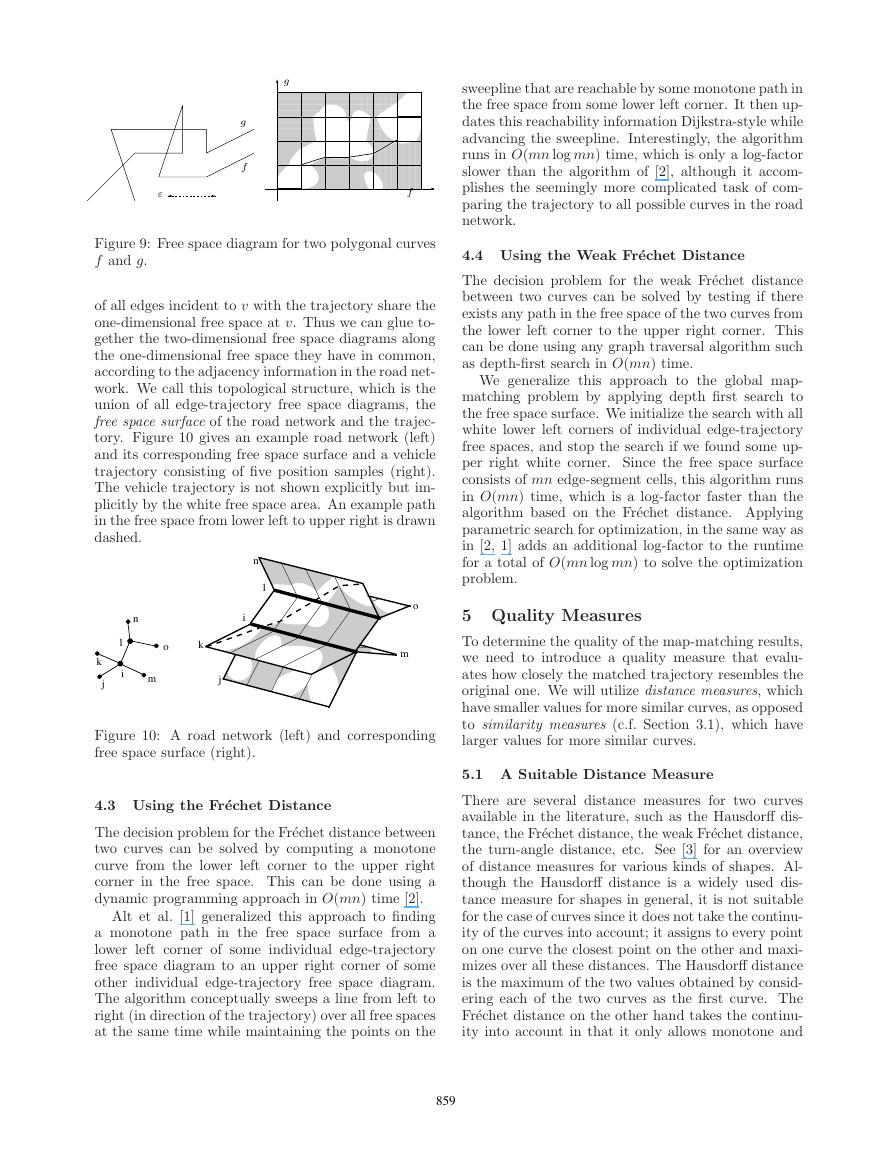The partition of [0, 1]2 into regions be- longing or not belonging to Fε(f, g) is called the free space diagram. Figure 9 shows polygonal curves f, g, a distance ε, and the corresponding free space diagram with the free space Fε = Fε(f, g) indicated in white. A monotone curve from the lower left corner to the upper right corner is drawn in the free space. This illustration is taken from [2]. The free space of two line segments is an ellipse [2] and the free space di- agram of two polygonal curves of m and n segments is composed of mn segment-segment free space dia- grams. In [2] it has been shown that δF(f, g) ≤ ε if and only if there exists a curve within Fε(f, g) from the lower left corner (0, 0) to the upper right corner (1, 1), which is monotone in both coordinates. Observe that the monotone curve in Fε(f, g) from the lower left corner to the upper right corner as a continuous mapping from [0, 1] to [0, 1]2 directly gives continuous non-decreasing reparametrizations α and β. Similarly, ˜δF(f, g) ≤ ε if and only if there exists a curve within Fε(f, g) from the lower left corner to the upper right corner, which is not necessarily monotone. The deﬁnition of the free space between two curves generalizes to the free space between an embedded graph and a curve as follows: The free space of the road network and the trajectory is the union of all free spaces of all straight-line edges of the road net- work with the vehicle trajectory. Notice that the free space of a vertex v with the vehicle trajectory is a one- dimensional free space, and the individual free spaces 858

g g f ε f Figure 9: Free space diagram for two polygonal curves f and g. of all edges incident to v with the trajectory share the one-dimensional free space at v. Thus we can glue to- gether the two-dimensional free space diagrams along the one-dimensional free space they have in common, according to the adjacency information in the road net- work. We call this topological structure, which is the union of all edge-trajectory free space diagrams, the free space surface of the road network and the trajec- tory. Figure 10 gives an example road network (left) and its corresponding free space surface and a vehicle trajectory consisting of ﬁve position samples (right). The vehicle trajectory is not shown explicitly but im- plicitly by the white free space area. An example path in the free space from lower left to upper right is drawn dashed. n l i n l i k j o k m j o m Figure 10: A road network (left) and corresponding free space surface (right). 4.3 Using the Fr´echet Distance The decision problem for the Fr´echet distance between two curves can be solved by computing a monotone curve from the lower left corner to the upper right corner in the free space. This can be done using a dynamic programming approach in O(mn) time [2]. Alt et al. [1] generalized this approach to ﬁnding a monotone path in the free space surface from a lower left corner of some individual edge-trajectory free space diagram to an upper right corner of some other individual edge-trajectory free space diagram. The algorithm conceptually sweeps a line from left to right (in direction of the trajectory) over all free spaces at the same time while maintaining the points on the sweepline that are reachable by some monotone path in the free space from some lower left corner. It then up- dates this reachability information Dijkstra-style while advancing the sweepline. Interestingly, the algorithm runs in O(mn log mn) time, which is only a log-factor slower than the algorithm of [2], although it accom- plishes the seemingly more complicated task of com- paring the trajectory to all possible curves in the road network. 4.4 Using the Weak Fr´echet Distance The decision problem for the weak Fr´echet distance between two curves can be solved by testing if there exists any path in the free space of the two curves from the lower left corner to the upper right corner. This can be done using any graph traversal algorithm such as depth-ﬁrst search in O(mn) time. We generalize this approach to the global map- matching problem by applying depth ﬁrst search to the free space surface. We initialize the search with all white lower left corners of individual edge-trajectory free spaces, and stop the search if we found some up- per right white corner. Since the free space surface consists of mn edge-segment cells, this algorithm runs in O(mn) time, which is a log-factor faster than the algorithm based on the Fr´echet distance. Applying parametric search for optimization, in the same way as in [2, 1] adds an additional log-factor to the runtime for a total of O(mn log mn) to solve the optimization problem. 5 Quality Measures To determine the quality of the map-matching results, we need to introduce a quality measure that evalu- ates how closely the matched trajectory resembles the original one. We will utilize distance measures, which have smaller values for more similar curves, as opposed to similarity measures (c.f. Section 3.1), which have larger values for more similar curves. 5.1 A Suitable Distance Measure There are several distance measures for two curves available in the literature, such as the Hausdorﬀ dis- tance, the Fr´echet distance, the weak Fr´echet distance, the turn-angle distance, etc. See [3] for an overview of distance measures for various kinds of shapes. Al- though the Hausdorﬀ distance is a widely used dis- tance measure for shapes in general, it is not suitable for the case of curves since it does not take the continu- ity of the curves into account; it assigns to every point on one curve the closest point on the other and maxi- mizes over all these distances. The Hausdorﬀ distance is the maximum of the two values obtained by consid- ering each of the two curves as the ﬁrst curve. The Fr´echet distance on the other hand takes the continu- ity into account in that it only allows monotone and 859

分享到：

赞收藏

资料库

On Map Matching Vehicle Tracking Data.pdf )

相关推荐

行业

热门标签

最新资料