Problem Chosen
A
2020
MCM/ICM
Summary Sheet
Team Control Number
2001334
Forecasts for the Ecology and Fisheries Economy of Scottish
herring and mackerel
As the favorable food for Scotch, the herring and mackerel bring generous profits to fishing
companies. Due to the hotter ocean, more fish move to the north to seek better habitats, laying a
negative impact on the fishing industry. The aim of this report is to build a migratory prediction
model to evaluate the influences on the income of fishing companies. We are expected to provide
some strategies for fishing companies who can adapt to the migration of fish under the constraints of
various objective conditions and prevent themselves from going bankrupt as much as possible. Three
models are established: Model I: Seawater Temperature Prediction Model; Model II: Fish Migration
Prediction Model; Model III: Fishing Company Earnings Evaluation Model.
For Model I, global ocean temperature date monthly from 1960 to 2019 is firstly collected. Then,
based on the analysis of intrinsic trend of the data and the verification of the stationarity, the validation
of using ARIMA model to predict temperature is proved. Next, historical data is used to fit the
parameters of ARIMA, with introduction of k-fold cross validation to identify the final prediction
model as ARIMA(1,1,0). Finally, according to ARIMA(1,1,0), bootstrap method is used to simulate
10000 possible prediction cases, which lays a great foundation to predict the migration of fish.
For Model II, firstly, according to the data of the migration speed and the ocean temperature, it is
determined that the temperature gradient is the main factor affecting the migration speed and direction.
And the corresponding empirical equation is established to determine the impact of temperature on
fish migration. Then based on the 10000 temperature change samples generated by bootstrap method
in Model I, migration situation of each sample is simulated to identify the most likely locations of the
fish. It was finally shown that the fish are mainly distributed in the area between Iceland and the Faroe
Islands 50 years later and the results are shown in figure 9.
For Model III, the profit evaluation equation of fishing companies is determined by the economic
principle, and the parameters involved are estimated by introducing the actual management data, the
results are shown in table 4; then based on the 10000 samples of fish migration from Model II, the
profit change of fishing companies is simulated for each sample and the profit trend over time is shown
in figure 10. Finally, it can be seen that the worst case is in 2030, fishing companies will go bankrupt
due to fish migration with a probability of 0.02%, the best case is that they will not go bankrupt in 50
years with a probability of 5.27% and the most likely case is that in 2039, fishing companies will go
bankrupt due to fish migration with a probability of 8.25%.
In addition, this report discusses the effective response to the fish migration for small fishing
companies, together with effective response strategies. Without considering the policies and legal
issues brought by the territorial sea, small fishing companies should transfer their ports to Iceland,
which is closer to the fish. Finally, based on simulation of this strategys effect, 100.00% of companies
can avoid bankruptcy. As for considering the policies and legal issues, small fishing companies should
upgrade their fishing vessels to extend the shelf life of fish. After simulation, 62.68% of companies
can avoid bankruptcy.
Eventually, robustness and sensitivity analysis of the model are tested. When the initial distribu-
tion of the fish is randomly generated from the uniform random distribution, the final convergence
distribution of the model has little difference. As for the factors that affect the model, social profit rate
and fishing boat navigation radius, it is found that the increase of these two factors will significantly
reduce the bankruptcy probability of fishing companies.
Keywords: ARIMA; Fish Migration; Earnings Evaluation; Computer Simulation
�
Team # 2001334
Team # 2001334
Team # 2001334
Page 1 of 27
Page 1 of 27
Page 1 of 27
Contents
.
.
.
.
.
.
.
.
.
.
.
.
.
.
.
.
.
.
.
.
.
.
.
.
.
.
.
.
.
.
. .
.
.
.
3.2.1 Data Collection .
3.2.2 Data Cleaning . .
. . . . . . . . . . . . . . . . . . . . . . . . . . . . . . .
1 Introduction . .
.
.
. . . . . . . . . . . . . . . . . . . . . . . . . . . . . .
1.1 Problem Background . .
1.2 Restatement of the Problem . . . . . . . . . . . . . . . . . . . . . . . . . . . . .
1.3 Our Approach . .
. . . . . . . . . . . . . . . . . . . . . . . . . . . . . .
2 General Assumptions and Model Overview . . . . . . . . . . . . . . . . . . . . . .
.
3 Model Preparation . .
. . . . . . . . . . . . . . . . . . . . . . . . . . . . . .
. . . . . . . . . . . . . . . . . . . . . . . . . . . . . . .
.
3.1 Notations . .
3.2 The Data . .
.
. . . . . . . . . . . . . . . . . . . . . . . . . . . . . . .
. . . . . . . . . . . . . . . . . . . . . . . . . . . . . .
.
.
. . . . . . . . . . . . . . . . . . . . . . . . . . . . . .
3.3 Geographic Coordinate System . . . . . . . . . . . . . . . . . . . . . . . . . . .
4 Model I: Seawater Temperature Prediction Model . . . . . . . . . . . . . . . . . . .
4.1 Description of Temperature Field . . . . . . . . . . . . . . . . . . . . . . . . . .
4.2 Autoregressive Prediction Model . . . . . . . . . . . . . . . . . . . . . . . . . .
. . . . . . . . . . . . . . . . . . . . . . . . . . . . . .
4.3 Results . .
4.3.1 Parameter Estimation . . . . . . . . . . . . . . . . . . . . . . . . . . . .
4.3.2 Calaculation Results . . . . . . . . . . . . . . . . . . . . . . . . . . . . .
5 Model II: Fish Migration Prediction Model . . . . . . . . . . . . . . . . . . . . . . .
5.1 Kinematics of Migration . . . . . . . . . . . . . . . . . . . . . . . . . . . . . . .
.
5.2 Kinetics of Migration . .
. . . . . . . . . . . . . . . . . . . . . . . . . . . . . .
. . . . . . . . . . . . . . . . . . . . . . . . . . . . . .
. .
5.3 Results . .
5.3.1 Estimation of ∇u .
. . . . . . . . . . . . . . . . . . . . . . . . . . . . . .
5.3.2 Estimation of f (∇u; v) . . . . . . . . . . . . . . . . . . . . . . . . . . . .
5.3.3 Migration Simulation Algorithm . . . . . . . . . . . . . . . . . . . . . .
5.3.4 Calaculation Results . . . . . . . . . . . . . . . . . . . . . . . . . . . . .
6 Model III: Fishing Company Earnings Evaluation Model . . . . . . . . . . . . . . .
. . . . . . . . . . . . . . . . . . . . . . . .
6.1 Fishing Company Operating Model
6.1.1 Assessment of Fishing Costs
. . . . . . . . . . . . . . . . . . . . . . . .
6.1.2 Assessment of Fishing Income . . . . . . . . . . . . . . . . . . . . . . .
. . . . . . . . . . . . . . . . . . . . . . . .
6.1.3 Assessment of Fishing Profit
. . . . . . . . . . . . . . . . . . . . . . . . . . . . . .
6.2.1 Parameter Estimation . . . . . . . . . . . . . . . . . . . . . . . . . . . .
6.2.2 Migration Simulation Algorithm . . . . . . . . . . . . . . . . . . . . . .
6.2.3 Calaculation Results . . . . . . . . . . . . . . . . . . . . . . . . . . . . .
. . . . . . . . . . . . . . . . . . . . . . . . . . . . . . .
6.3.1 The Management Strategies without Consider of Territorial Sea . . . .
6.3.2 The Management Strategies with Consider of Territorial Sea . . . . . .
. . . . . . . . . . . . . . . . . . . . . . . . . . . . . . .
. . . . . . . . . . . . . . . . . . . . . . . . . . . . . .
.
6.3 Discussion .
6.2 Results . .
. .
. .
7 Test the Model
.
7.1 Sensitivity Analysis . .
. .
.
.
.
.
.
.
.
.
.
.
.
.
.
.
.
.
.
.
.
.
.
.
.
.
.
.
1
1
1
1
2
3
3
3
4
4
4
5
5
5
7
7
7
8
8
9
9
9
9
10
10
11
11
11
11
11
11
11
12
13
14
14
15
16
16
�
.
.
.
.
.
.
.
. .
.
.
7.2 Robustness Analysis . .
8 Conclusion . .
.
8.1 Summary of Results . .
. . . . . . . . . . . . . . . . . . . . . . . . . . . . . .
. . . . . . . . . . . . . . . . . . . . . . . . . . . . . .
. . . . . . . . . . . . . . . . . . . . . . . . . . . . . .
8.1.1 Result of Problem 1 . . . . . . . . . . . . . . . . . . . . . . . . . . . . . .
8.1.2 Result of Problem 2 . . . . . . . . . . . . . . . . . . . . . . . . . . . . . .
8.1.3 Result of Problem 3 . . . . . . . . . . . . . . . . . . . . . . . . . . . . . .
8.1.4 Result of Problem 4 . . . . . . . . . . . . . . . . . . . . . . . . . . . . . .
. . . . . . . . . . . . . . . . . . . . . . . . . . . . . . .
8.2 Strength . .
.
. . . . . . . . . . . . . . . . . . . . . . . . . . . . . .
.
8.3 Possible Improvements .
. .
. . . . . . . . . . . . . . . . . . . . . . . . . . . . . .
References . .
Appendices .
. . . . . . . . . . . . . . . . . . . . . . . . . . . . . .
. .
Appendix A Tools and software . . . . . . . . . . . . . . . . . . . . . . . . . . . . . .
Appendix B The Codes .
. . . . . . . . . . . . . . . . . . . . . . . . . . . . . .
B.1 ARIMA Model Parameter Estimation and Ordering Code . . . . . . . . . . . .
B.2 Bootstrap Simulation Codes . . . . . . . . . . . . . . . . . . . . . . . . . . . . .
. .
. .
.
.
. .
.
.
.
.
.
.
.
.
.
.
.
. .
.
.
.
.
.
.
.
17
17
17
17
18
19
19
20
20
20
22
22
22
22
24
�
Team # 2001334
Team # 2001334
Team # 2001334
1 Introduction
1.1 Problem Background
Page 1 of 27
Page 1 of 27
Page 1 of 27
Global ocean temperatures affect the quality of habitats for certain ocean-dwelling species.
When temperature changes are too great for their continued thriving, these species move to
seek other habitats better suited to their present and future living and reproductive success.
The consortium wants to gain a better understanding of issues related to the potential migra-
tion of Scottish herring and mackerel from their current habitats near Scotland if and when
global ocean temperatures increase. These two fish species represent a signficant economic
contribution to the Scottish fishing industry. Changes in population locations of herring and
mackerel could make it economically impractical for smaller Scotland-based fishing com-
panies, who use fishing vessels without on-board refrigeration, to harvest and deliver fresh
fish to markets in Scotland fishing ports.
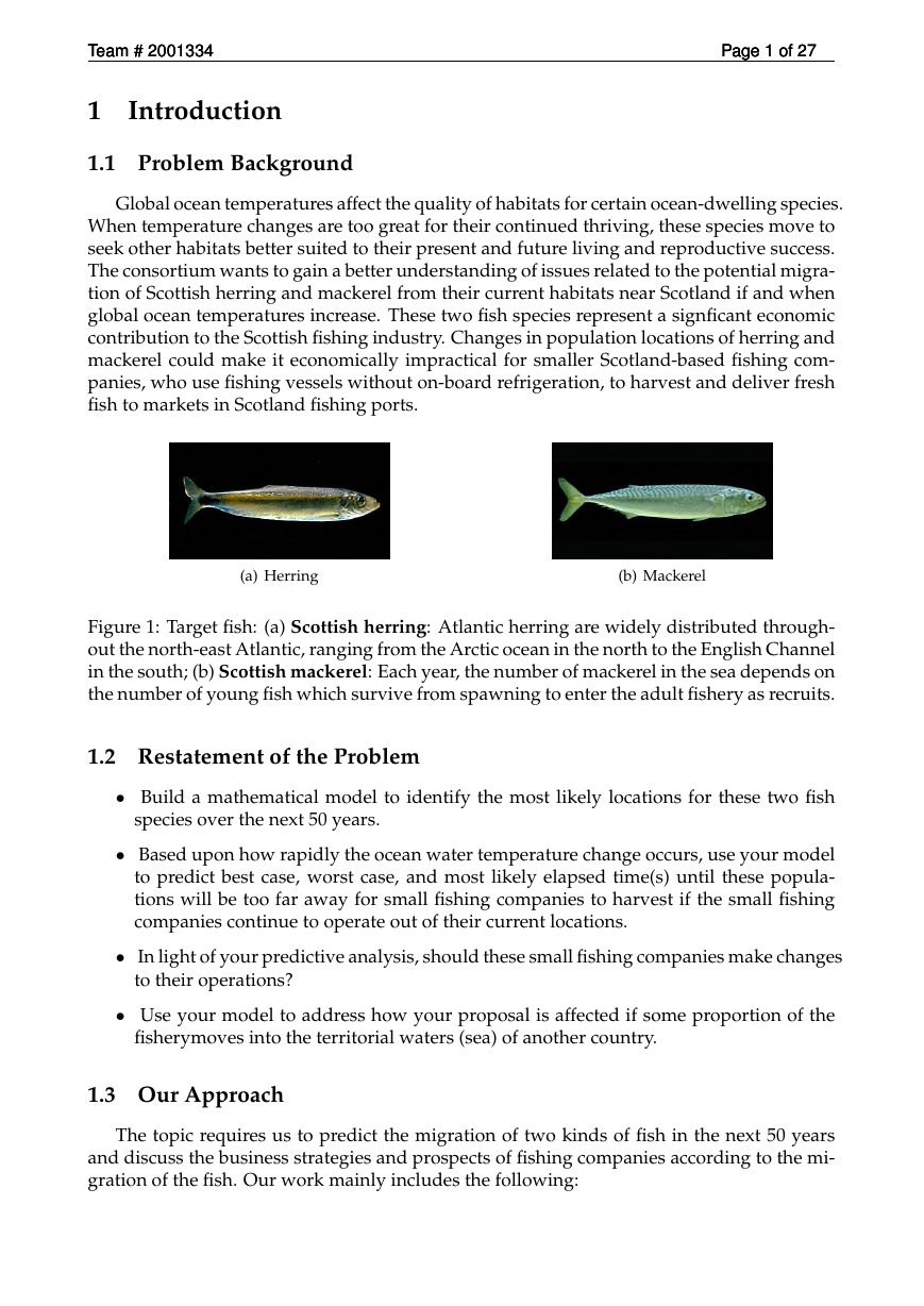
(a) Herring
(b) Mackerel
Figure 1: Target fish: (a) Scottish herring: Atlantic herring are widely distributed through-
out the north-east Atlantic, ranging from the Arctic ocean in the north to the English Channel
in the south; (b) Scottish mackerel: Each year, the number of mackerel in the sea depends on
the number of young fish which survive from spawning to enter the adult fishery as recruits.
1.2 Restatement of the Problem
• Build a mathematical model to identify the most likely locations for these two fish
species over the next 50 years.
• Based upon how rapidly the ocean water temperature change occurs, use your model
to predict best case, worst case, and most likely elapsed time(s) until these popula-
tions will be too far away for small fishing companies to harvest if the small fishing
companies continue to operate out of their current locations.
• In light of your predictive analysis, should these small fishing companies make changes
to their operations?
• Use your model to address how your proposal is affected if some proportion of the
fisherymoves into the territorial waters (sea) of another country.
1.3 Our Approach
The topic requires us to predict the migration of two kinds of fish in the next 50 years
and discuss the business strategies and prospects of fishing companies according to the mi-
gration of the fish. Our work mainly includes the following:
�
Team # 2001334
Team # 2001334
Team # 2001334
Page 2 of 27
Page 2 of 27
Page 2 of 27
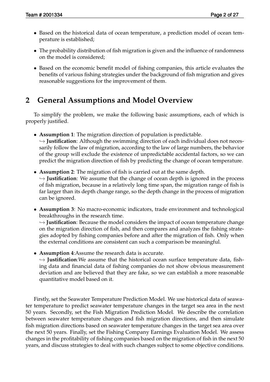
• Based on the historical data of ocean temperature, a prediction model of ocean tem-
perature is established;
• The probability distribution of fish migration is given and the influence of randomness
on the model is considered;
• Based on the economic benefit model of fishing companies, this article evaluates the
benefits of various fishing strategies under the background of fish migration and gives
reasonable suggestions for the improvement of them.
2 General Assumptions and Model Overview
To simplify the problem, we make the following basic assumptions, each of which is
properly justified.
• Assumption 1: The migration direction of population is predictable.
,→ Justification: Although the swimming direction of each individual does not neces-
sarily follow the law of migration, according to the law of large numbers, the behavior
of the group will exclude the existence of unpredictable accidental factors, so we can
predict the migration direction of fish by predicting the change of ocean temperature.
• Assumption 2: The migration of fish is carried out at the same depth.
,→ Justification: We assume that the change of ocean depth is ignored in the process
of fish migration, because in a relatively long time span, the migration range of fish is
far larger than its depth change range, so the depth change in the process of migration
can be ignored.
• Assumption 3: No macro-economic indicators, trade environment and technological
breakthroughs in the research time.
,→ Justification: Because the model considers the impact of ocean temperature change
on the migration direction of fish, and then compares and analyzes the fishing strate-
gies adopted by fishing companies before and after the migration of fish. Only when
the external conditions are consistent can such a comparison be meaningful.
• Assumption 4:Assume the research data is accurate.
,→ Justification:We assume that the historical ocean surface temperature data, fish-
ing data and financial data of fishing companies do not show obvious measurement
deviation and are believed that they are fake, so we can establish a more reasonable
quantitative model based on it.
Firstly, set the Seawater Temperature Prediction Model. We use historical data of seawa-
ter temperature to predict seawater temperature changes in the target sea area in the next
50 years. Secondly, set the Fish Migration Prediction Model. We describe the correlation
between seawater temperature changes and fish migration directions, and then simulate
fish migration directions based on seawater temperature changes in the target sea area over
the next 50 years. Finally, set the Fishing Company Earnings Evaluation Model. We assess
changes in the profitability of fishing companies based on the migration of fish in the next 50
years, and discuss strategies to deal with such changes subject to some objective conditions.
�
Team # 2001334
Team # 2001334
Team # 2001334
Page 3 of 27
Page 3 of 27
Page 3 of 27
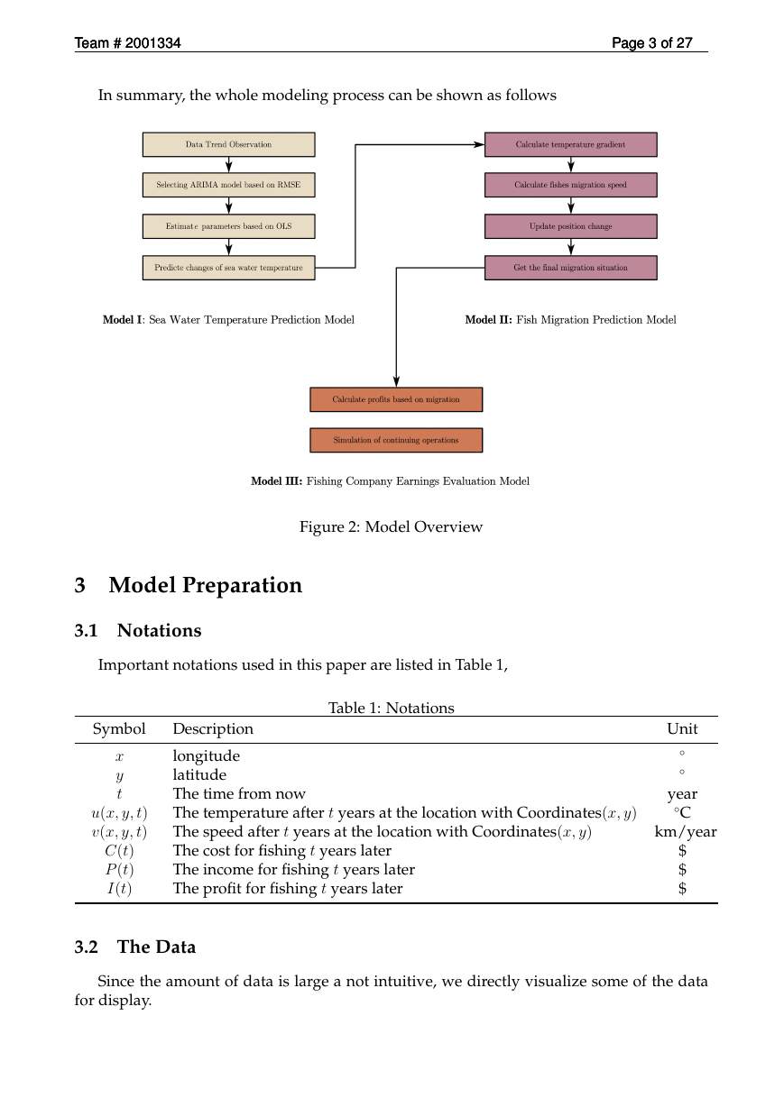
In summary, the whole modeling process can be shown as follows
Figure 2: Model Overview
3 Model Preparation
3.1 Notations
Important notations used in this paper are listed in Table 1,
Table 1: Notations
Symbol
x
y
t
u(x; y; t)
v(x; y; t)
C(t)
P (t)
I(t)
Description
longitude
latitude
The time from now
The temperature after t years at the location with Coordinates(x; y)
The speed after t years at the location with Coordinates(x; y)
The cost for fishing t years later
The income for fishing t years later
The profit for fishing t years later
Unit
◦
◦
year
◦C
km/year
$
$
$
3.2 The Data
Since the amount of data is large a not intuitive, we directly visualize some of the data
for display.
�
Team # 2001334
Team # 2001334
Team # 2001334
3.2.1 Data Collection
Page 4 of 27
Page 4 of 27
Page 4 of 27
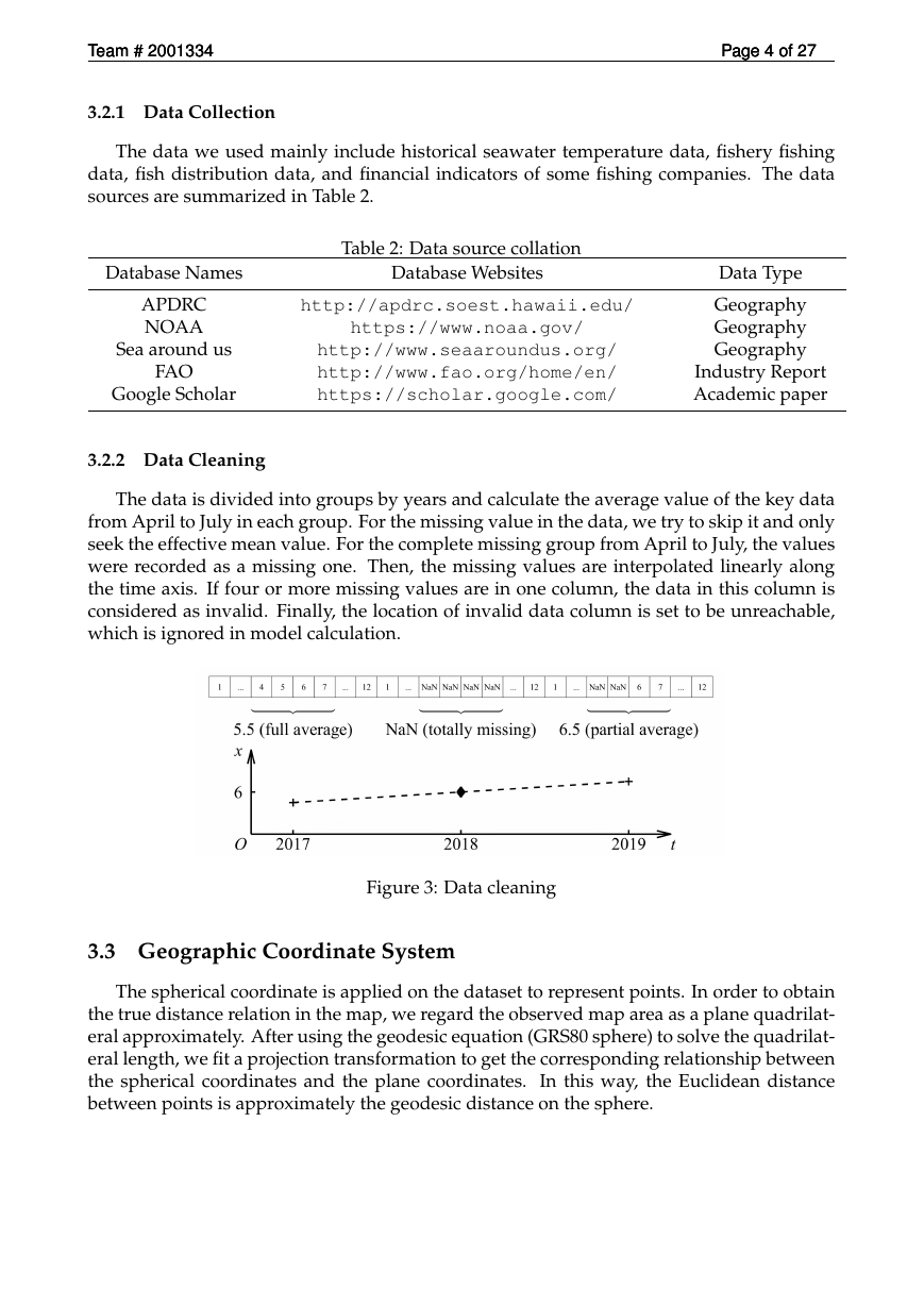
The data we used mainly include historical seawater temperature data, fishery fishing
data, fish distribution data, and financial indicators of some fishing companies. The data
sources are summarized in Table 2.
Database Names
APDRC
NOAA
Sea around us
FAO
Google Scholar
Table 2: Data source collation
Database Websites
http://apdrc.soest.hawaii.edu/
https://www.noaa.gov/
http://www.seaaroundus.org/
http://www.fao.org/home/en/
https://scholar.google.com/
Data Type
Geography
Geography
Geography
Industry Report
Academic paper
3.2.2 Data Cleaning
The data is divided into groups by years and calculate the average value of the key data
from April to July in each group. For the missing value in the data, we try to skip it and only
seek the effective mean value. For the complete missing group from April to July, the values
were recorded as a missing one. Then, the missing values are interpolated linearly along
the time axis. If four or more missing values are in one column, the data in this column is
considered as invalid. Finally, the location of invalid data column is set to be unreachable,
which is ignored in model calculation.
Figure 3: Data cleaning
3.3 Geographic Coordinate System
The spherical coordinate is applied on the dataset to represent points. In order to obtain
the true distance relation in the map, we regard the observed map area as a plane quadrilat-
eral approximately. After using the geodesic equation (GRS80 sphere) to solve the quadrilat-
eral length, we fit a projection transformation to get the corresponding relationship between
the spherical coordinates and the plane coordinates.
In this way, the Euclidean distance
between points is approximately the geodesic distance on the sphere.
�
Team # 2001334
Team # 2001334
Team # 2001334
Page 5 of 27
Page 5 of 27
Page 5 of 27
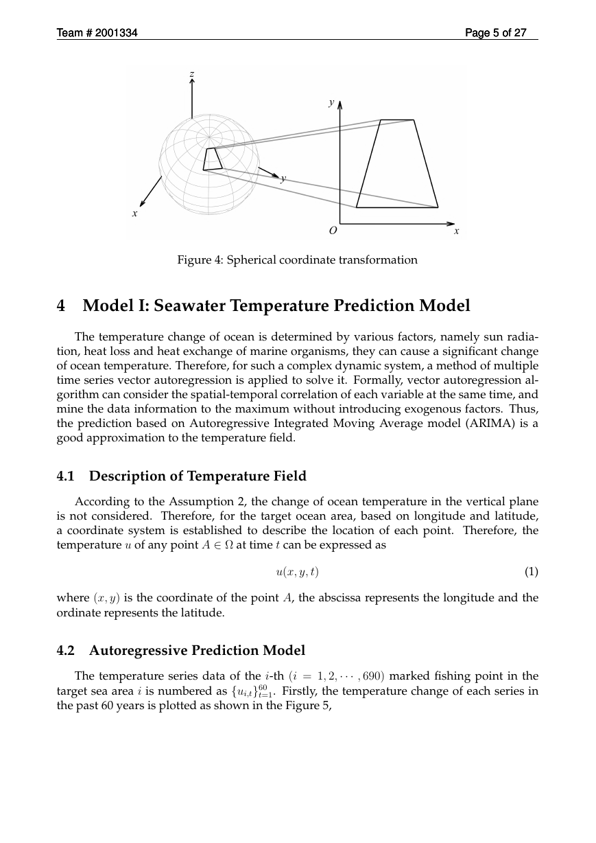
Figure 4: Spherical coordinate transformation
4 Model I: Seawater Temperature Prediction Model
The temperature change of ocean is determined by various factors, namely sun radia-
tion, heat loss and heat exchange of marine organisms, they can cause a significant change
of ocean temperature. Therefore, for such a complex dynamic system, a method of multiple
time series vector autoregression is applied to solve it. Formally, vector autoregression al-
gorithm can consider the spatial-temporal correlation of each variable at the same time, and
mine the data information to the maximum without introducing exogenous factors. Thus,
the prediction based on Autoregressive Integrated Moving Average model (ARIMA) is a
good approximation to the temperature field.
4.1 Description of Temperature Field
According to the Assumption 2, the change of ocean temperature in the vertical plane
is not considered. Therefore, for the target ocean area, based on longitude and latitude,
a coordinate system is established to describe the location of each point. Therefore, the
temperature u of any point A ∈ Ω at time t can be expressed as
u(x; y; t)
(1)
where (x; y) is the coordinate of the point A, the abscissa represents the longitude and the
ordinate represents the latitude.
4.2 Autoregressive Prediction Model
The temperature series data of the i-th (i = 1; 2;··· ; 690) marked fishing point in the
t=1. Firstly, the temperature change of each series in
target sea area i is numbered as {ui,t}60
the past 60 years is plotted as shown in the Figure 5,
�


 2023年江西萍乡中考道德与法治真题及答案.doc
 2012年重庆南川中考生物真题及答案.doc
 2013年江西师范大学地理学综合及文艺理论基础考研真题.doc
 2020年四川甘孜小升初语文真题及答案I卷.doc
 2020年注册岩土工程师专业基础考试真题及答案.doc
 2023-2024学年福建省厦门市九年级上学期数学月考试题及答案.doc
 2021-2022学年辽宁省沈阳市大东区九年级上学期语文期末试题及答案.doc
 2022-2023学年北京东城区初三第一学期物理期末试卷及答案.doc
 2018上半年江西教师资格初中地理学科知识与教学能力真题及答案.doc
 2012年河北国家公务员申论考试真题及答案-省级.doc
 2020-2021学年江苏省扬州市江都区邵樊片九年级上学期数学第一次质量检测试题及答案.doc
 2022下半年黑龙江教师资格证中学综合素质真题及答案.doc