Bayesian Channel Estimation for Massive MIMO Communications Chengzhi Zhu, Zhitan Zheng, Bin Jiang, Wen Zhong, and Xiqi Gao National Mobile Communications Research Laboratory, Southeast University, Nanjing 210096, P. R. China Email: {bjiang, xqgao}@seu.edu.cn Abstract—In this paper, we derive the Bayes-Optimal estimator based on approximate message passing (AMP) algorithm in massive multiple-input multiple-output (MIMO) systems, which requires statistical channel state information (CSI). According to the analysis of channel model in beam domain, the convariance matrix is derived for CSI acquisition. With the aid of statistical CSI, the convergence of the proposed algorithm has significant improvement in comparison with which use the expectation- maximization (EM) algorithm to fit the statistical CSI. Sim- ulations show great mean squared error (MSE) performance that approximates the Minimum Mean Square Error (MMSE) estimator, and better convergence performance than other AMP algorithm can be achieved. Besides, the results prove that performance of the random pilot in this algorithm is close to that of the orthogonal pilot based on Zadoff-Chu sequences. I. INTRODUCTION Massive MIMO systems, which employ a large number of antennas at the base station (BS) to simultaneously serve a relatively large number of users [1], are believed to be one of the key candidate technologies for forthcoming 5G wireless networks [2], [3] with the potential large gains in spectral efficiency and energy efficiency. Channel state information which is typically obtained with the assistance of the periodically inserted pilot signals [4], plays a significant role in massive MIMO transmission. CSI makes it possible to adapt transmissions to current channel conditions, which is crucial for achieving robust communica- tion in massive MIMO systems. Due to the fact that statistical CSI varies over much longer time scales than instantaneous CSI, we use statistical CSI instead of instantaneous CSI. And more importantly, statistical CSI requires much less over- head. MIMO channel estimation based on Gaussian-Mixture Bayesian learning has been investigated in [5], [6]. Instead of using expectation-maximization (EM) [5]–[7] algorithm to learn the channel properties, we use statistical CSI as known properties to reduce the complexity and improve the perfor- mance of AMP algorithm. In massive MIMO systems, accurate statistical CSI is required not only in channel estimation, but also in other aspects [8], [9], such as user scheduling . In this work, we model each channel element in the beam domain as a Gaussian variable. This model enables a more accurate learning of AMP algorithm, in comparison with Gaussian-Mixture. We can reconstruct the channel components with great mean-squared error (MSE) performance which is close to LMMSE channel estimation. Throughout this paper, we use the following notation: C denotes the set of complex numbers. We use ai;j to denote the (i; j)th element of matrix A. AT denotes the transpose of A and AH denotes the conjugate transpose of A. Identity matrix is denoted by IK. E{·} represents the expectation operation. x ∼ NC(; 2) denotes a random complex variable x comply with the complex Gaussian distribution with mean and variance 2, where ( −|x − |2 ) : 2 fX (x) = 1 2 exp II. SYSTEM MODEL We consider single-cell TDD massive MIMO wireless trans- mission scheme which consists of one BS equipped with N antennas and K single-antenna users. Assume that the BS is equipped with a uniform linear array (ULA), and the antennas are separated by half wavelength. We assume that the uplink pilot S ∈ CL×K where L denotes the pilot length. We use hk;n to represent the channel coefficient of kth user and nth beam in the beam domain [8]. With these definitions, the received signal of the lth symbol in the nth beam can be written as sl;khk;n + zl;n = sT l hn + zl;n; (1) K∑ yl;n = k=1 where sl;k represents lth symbol of the kth user’s pilot signal, zl;n is the Gaussian noise in the beam domain with zero mean z, sl = [sl;1; sl;2; :::sl;K]T , and hn ∈ CK×1 is and variance 2 the channel vector of all users in the nth beam. Let gk = [hk;1; hk;2; :::; hk;N ]T . According to [8]–[10], the uplink channel of kth user can be modeled as ∫ gk = vk a()rk()d; (2) A where a () = [1; exp(−j sin()); :::; exp(−j(N − 1) sin())]T is the ULA response vector [10], A = [−=2; =2] is the (AOA), vk ∼ NC (0; IN ) and rk() angle of arrival denotes the channel gain function. We assume that the channel phases are uniformly distirbuted, thus E{gk} = 0, i.e., and different beams of channels are uncorrelated, E{rk()rH ) [9]. Let Rk denotes k ( channel covariance matrix: Rk = E{gkgH } = )} = Sk()( − a()aH()Sk()d: ∫ (3) k ′ ′ A 

Note that k is a diagonal matrix satisfying [k]nn = Sk(n). Then gk can be rewritten as = 2 AS Note that Sk () represents the channel power azimuth spread (PAS) which can be modeled as the truncated Laplacian distribution [11]: 1√ 2AS − ¯ √ 2 AS )·exp 1 1 − exp (√ Sk () = ( ) (4) − · where −=2 ≤ ≤ =2 and AS denotes the azimuth spread (AS). We assume that the users are uniformly distributed and the mean channel AOA ¯ is uniformly distributed in the angle interval [−=2; =2]. − 1); n = 0; 1; 2; :::; N − 1. When N Let n = arcsin( 2n N is sufficiently large, the eigenvector of the channel covariance matrix can be well approximated by the unitary DFT matrix [9], which is denoted as F ∈ CN×N . The channel covariance matrix can be well approximated by Rk = FkFH : (5) gk = vkF 1 2 k : (6) It can be found that the beam domain channel coefficient is approximately sparse [8], and its sparsity is related to its PAS. More specifically, over 95% of the channel power focus on less than 15% of the beam indexs. Moreover, we can see that the eigenvector is independent of beams. Thus, gk has d- ifferent covariance, i.e., k = diag , it means hk;n ∼ NC(0; 2 2 k;1; :::; 2 k;n; :::; 2 { } k;N k;n). III. BAYESIAN CHANNEL ESTIMATION The purpose of channel estimation is to reconstruct the beam domain channel coefficient hn from the received signal yn = [y1;n; :::; yl;n; :::; yL;n]T by given the pilot matrix S. Supposing that we adopt LS or MMSE channel estimator [10]– [12], we may come with the problem of the pilot contamina- tion and the nonorthogonal of pilots. Besides, LS or MMSE estimator can’t avoid large scale matrix inversion. When the number of users K linearly increases, the implementation complexity increases by K 3. In order to minimize the MSE of hk;n and to avoid the matrix inversion, we can perform the Bayes-optimal estimator [6], [13]: ∫ ˆhk;n = hk;nqk;n (hk;n) dhk;n (7) ∫ where qk;n (hk;n) is the marginal probability distribution func- tion (pdf) of P (hn|yn), i.e., qk;n (hk;n) = {hi;n} i̸=k P (hn|yn): (8) exp = 1 ∆ d exp − 2 ∆ + i2! ∆ : (13) Eq. (8) is known as the Nishimori conditions in the physics of disorder systems [6]. The directly computation of (8) is not tractable. However, it can be effectively estimated by using the AMP algorithm. and let ! = which is shown at the top of the page. 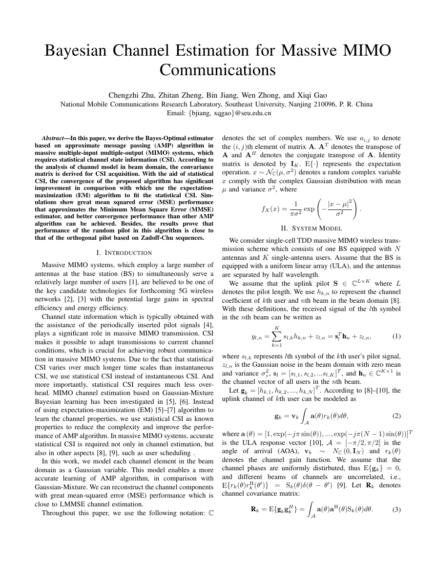j̸=k sl;jhj;n,then (11) can be simplified to (14), For a general complex Gaussian distribution with the mean the characteristic function can be and the variance , Fig. 1. A factor graph of Eq.(8). ) ( ( Before performing the Bayesian estimation, we need to fully k;n and the noise z which can be obtained by statistical channel state know the variances of the channel elements 2 level 2 information acquisition [8]. The pdf of yn is P (yn|hn) = L∏ 1 z )L exp (2 1 exp 2 z l=1 ∥yn − Shn∥2 ∑K yl;n − − 1 2 z − 1 2 z sl;khk;n k=1 ) 2 : (9) Then we can get the posterior probability distribution of hn: P (hn|yn) = = P (yn) P (yn|hn)P (hn) K∏ ( Z(yn; hn) k=1 1 L∏ 1 2 z exp l=1 P (hk;n)· yl;n − − 1 2 z ∑K k=1 sl;khk;n ) 2 (10) where Z(yn; hn) denotes the normalization factor. We can use factor graph [14], [15] to calculate P (yn|hn). ∏ In Fig. 1, we have messages passing from the observation nodes yn to the channel nodes hn, which can be described as ∫ ∏ dhj;nP (yl;n|hn) qj→l;n(hj;n); ql→k;n(hk;n) = 1 Zl→k j̸=k (11) and messages passing from the channel nodes hn to the observation nodes yn: j̸=k qk→l;n(hk;n) = P (hk;n) q→k;n(hk;n): (12) Note that both Zl→k and Zk→l are normalization factor to ensure qk→l;n(hk;n)dhk;n = 1. ql→k;n(hk;n)dhk;n = By using the complex form of Hubbard-Stratonovich trans- formation [16], i.e. , ) ∫ ∏ ̸=l ( 1 Zk→l ∫ ∫ ( ) − !2 ∆ ∑ 1,,knknqho,knh,lny. . .. . .,,kLnknqho,,lknknqho,|lnnPyh1,nPh,KnPh1,knh1,nh1,knh,Knh1,,knknqho1,ny,knh1,lny,lny,Lny1,lny. . .. . .,,Lknknqho,knPh,,klnknqho1,|nnPyh,|LnnPyh

∫ ql→k;n(hk;n) = · d exp · exp Zl→k 1 ∫ ∏ − 2 2 z j̸=k ( − 1 2 z |sl;khk;n − yl;n|2 ( ) qj→l;n(hj;n) exp 2sl;jhj;n (yl;n − sl;khk;n + i) 2 z ) dhj;n (14) ( ) ql→k;n(hk;n) = 1 · exp  2 Zl→k j̸=k sl;j (∑ − [ d exp · exp ∫ · ˆhj→t;n 2 z (∑ 2 z + j̸=k |sl;khk;n − yl;n|2 − 1 2 z (yl;n − sl;khk;n) )] + |sl;j|2j→l;n z )2 (2 ) (∑ (∑ j̸=k ) (yl;n − sl;khk;n)2 ) (∑  |sl;j|2j→l;n z )2 (2 ) 2 + ˆhj→l;n j̸=k sl;j 2 z i 2 + j̸=k |sl;j|2j→l;n z )2 (2 (yl;n − sl;khk;n) i  (16) (21) : 2 ) ( } = exp i! − 1 4 { E ei!x ∫ described as ∫ dhk;nh2 Let ˆhk→l;n = k;nqk→l;n(hk;n)−ˆh2 dhk;nhk;nqk→l;n(hk;n) and k→l;n = k→l;n be the mean and variance of qk→l;n(hk;n) respectively. Then (14) can be simplified to (16). Performing the integral over with the Hubbard- Stratonovich transformation, we obtain !22 : (15) ( − hk;n − Bl→k;n ) Al→k;n 1 Al→k;n )2  exp 1 Al→k;n 1 ( · −h2 k;n ql→k;n(hk;n) = = 1 ˜Zl→k;n exp where Al→k;n + 2Bl→k;nhk;n ; ) (17) (18) ( ∑ |sl;k|2 l;n −∑ j̸=k ∑ j̸=k l→k;n B2 Al→k;n : e 2 z + ∗ s l;k 2 z + Al→k;n |sl;j|2j→l;n ˆhj→l;n j̸=k sl;j |sl;j|2j→l;n Al→k;n = Bl→k;n = ˜Zl→k;n = Note that the normalization ˜Zl→k;n contains all the hk;n- independent factors, therefore (12) can be presented as 1 ˜Zk→l;n P (hk;n) ∑ ) A→k;n + 2hk;n ̸=l B→k;n ̸=l (19) The mean and variance of hk;n can also be given as (7) and k;n = dhk;nh2 k;nqk;n(hk;n)−ˆh2 k;n; (20) ( qk→l;n(hk;n) = · exp −h2 k;n ∑ ∫ We have Vk;n = to be the mean and variance of P (yn|hn) respectively. We can obtain and Uk;n = A→k;n then we can get ( qk;n(hk;n) = −h2 · exp k;n ∑ 1 ˜Zk;n [∑ [∑ [∑ [∑ · Uk;n = ≃ Vk;n ≃ =ˆhk→;n + where P (hk;n) ∑ A→k;n + 2hk;n ∑ B→k;n A→k;n ∑ ) B→k;n 1∑ ]−1 |s;k|2 ]−1 2 z + ;n ]−1 z + ;n − |s;k|2k→;n 2 |s;k|2 2 z + ;n ;k (y;n − !;n) + |s;k|2ˆhk→;n ∗ s |s;k|2 ∑ ∑ 2 z + ;n ∗ s ;k ∑ |s;k|2 ∑ (y;n−!;n) 2 z +;n |s;j|2j→;n ˆhj→;n: s;j ;n = !;n = j z +;n 2 1 j ] (22) (23) From the taylor expansion of ˆhk→l;n [6], we can neglect the terms that satisfies sc ∑ ∑ j j l;n = !l;n = Vk;n = ˆhk;n + l;n; c > 2. Then we get |sl;j|2j;n ˆhj;n − (yl;n − !l;n) ∑ ∑ 2 z + l;n (y;n−!;n) 2 z +;n ∗ s ;k |s;k|2 sl;j 1 : 2 z +;n l;n (24) 

The mean and variance of qk:n(hk;n) are P (hk;n|Vk;n) = ( P (Vk;n|hk;n)P (hk;n) P (Vk;n|hk;n)P (hk;n)dhk;n ) ∫ = NC 2 k;nVk;n 2 k;n + Uk;n ; Uk;n2 k;n 2 k;n + Uk;n (25) . and vk;n = Uk;n2 k;n 2 k;n+Uk;n The posterior mean and variance are represented as ˆhk;n = 2 k;nVk;n 2 k;n+Uk;n After a thorough analysis of these problems, we can come up with the proposed algorithm. Suppose that the variances of hn and zl;n can be obtained by statistical channel state information acquisition [8]. t = 0; 1; ::: denotes the iteration index. Then the learning progress for estimating hn is given as: Algorithm 1: The Proposed Algorithm Data: Input pilot matrix S = {sl;k}l=1;:::;L;k=1;:::;K and yn = {y1;n; :::; yL;n}T ∈ CL, Statistical CSI acquisition: 2 z. k;n and 2 Result: Return the beam domain channel hn. initialization: t = 1, l;n = yl;n; ˆh0 !0 for n = 1 to N do k;n = 0;∀l; k; n; k;n = 1; v0 repeat − ˆht−1 until number for iterations to reach. k;n k;n k < ", " is a predefined The complexity of the proposed algorithm is O(L + K) per iteration, which is obviously lower than that of MMSE estimation. IV. NUMERICAL RESULTS In this section, we give some examples to illustrate the advantages of the proposed algorithm in massive MIMO system. Our simulations are based on a single cell which is equipped with a 256-antenna ULA with half wavelength antenna spacing. The number of users is set to K = 80, and the pilot length satisfying L = K. 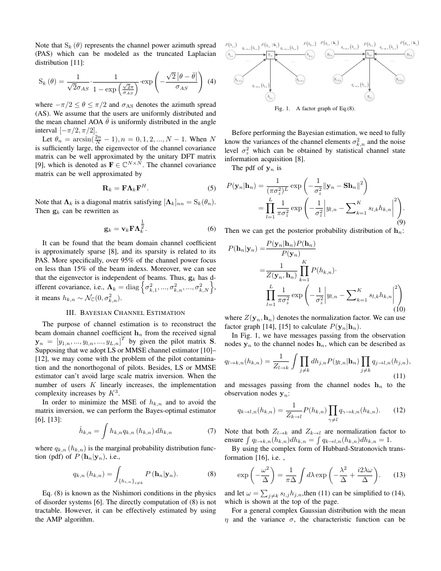The PAS of the users is ◦ and ¯ being uniformly distributed given by (4) with AS = 3 ∑ ∑ j;n; n = 1 j vt t+1 L for l = 1 to L do ˆht j;n !t+1 ∑ l;n = n = 2 j sl;j n ; z + t+1 U t+1 for k = 1 to K do k;n = ˆht V t+1 k;n + k;nV t+1 2 ˆht+1 k;n = k;n+U t+1 2 U t+1 k;n 2 k;n+U t+1 2 k;n k;n k;n k;n ; vt+1 k;n = ∑ t ← t + 1; ˆht 2 − (yl;n−!t z +t 2 l;n l;n) t+1 l;n ; ) y;n − !t+1 ;n ; ( ∗ s ;k ; Fig. 2. and different pilot types. The convergence of the proposed algorithm under different SNRs within [−90 ◦ pathloss between the BS and an UE at distance d is set to ]. For the sake of comparison with [5], the ◦ ; 90 with = 3:8. The normalized mean square error is defined as g(d) = 1 1 + d N∑ K∑ N∑ k−1 2 ˆhk;n − hk;n K∑ |hk;n|2 (26) (27) NMSE = 10 lg n=1 n=1 k=1 In this paper, we compare two different types of the pilot: { the orthogonal pilot and the random pilots. The orthogonal pilot sequences are generated from Zadoff-Chu sequence [17], using cyclic shift between users to ensure SH S = IK. The ran- dom pilot sequences are randomly generated from with equal probability, to make sure that |sk|2 = 1. A. Algorithm Convergence of Different Estimators ±√ } 1=L In this subsection, we discuss the algorithm convergence. Firstly, the performance of the two pilot sequences is given in Fig. 2. Fig. 2 shows how different pilot sequences and SNRs effect on the algorithm convergence. It is evident that the proposed algorithm with orthogonal pilot has a slight advantage against the other one. Noticing that although the convergence perfor- mance of the proposed algorithm degrades with higher SNR, this algorithm can still converge in about six iterations even under the SNR of 30dB. 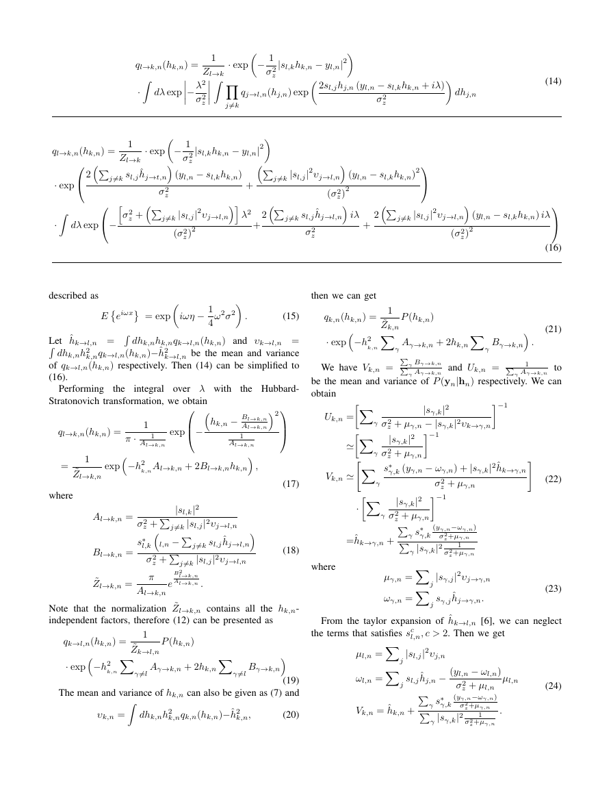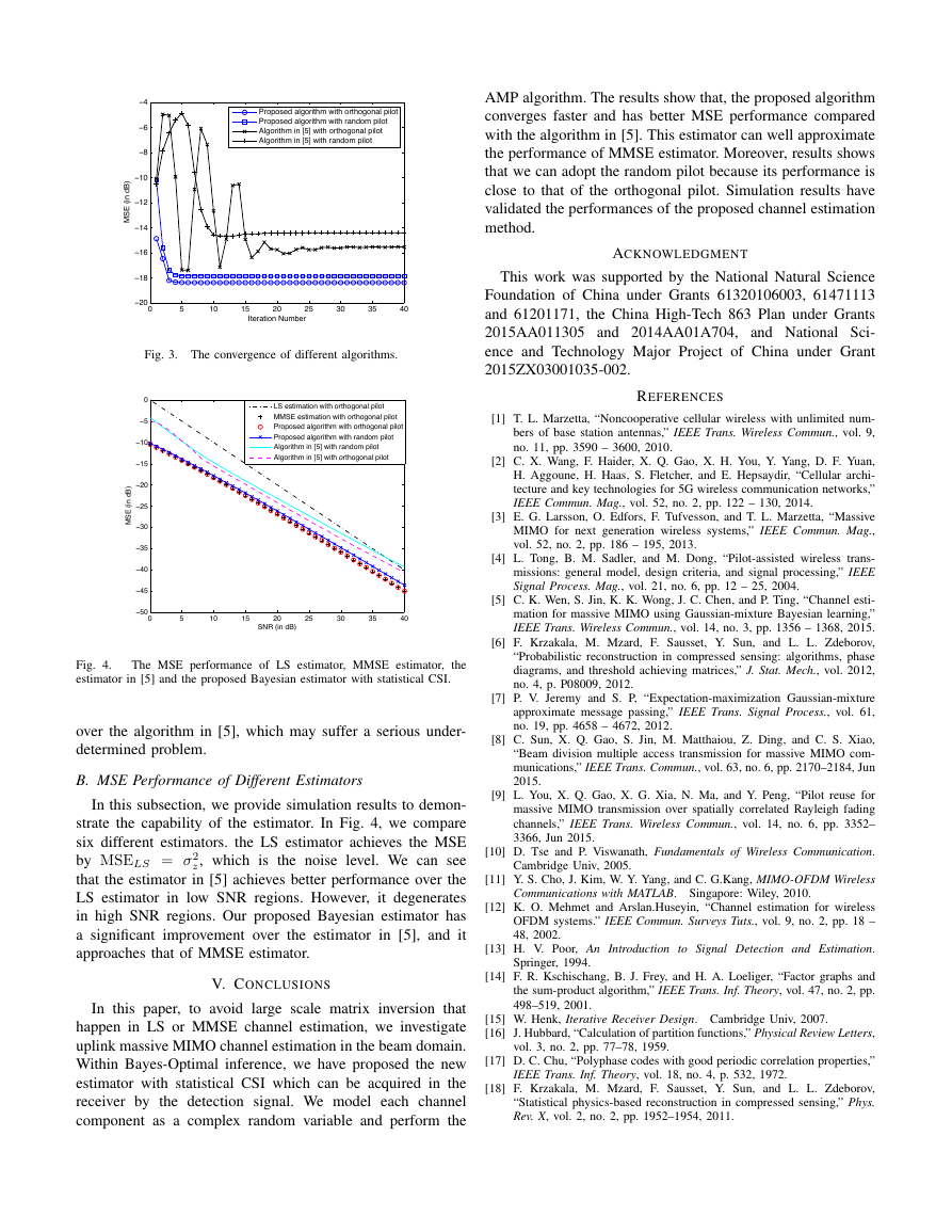In Fig. 3, we discuss the difference between the proposed algorithm and the algorithm in [5] which does not include accurate channel information [6], [18]. The algorithm in [5] models the channel as Gaussian mixture model, and has a better performance than the LS estimator. However, unknown channel information will complicates the algorithm. In this paper, we set three different variances for the algorithm in [5]. From Fig. 3, we can see that the proposed algorithm with statistical CSI is more stable and has a better performance 02468101214161820−40−35−30−25−20−15−10−5Iteration NumberMSE (in dB) Orthogonal pilotRandom pilotSNR = 10dBSNR = 20dBSNR = 30dB

AMP algorithm. The results show that, the proposed algorithm converges faster and has better MSE performance compared with the algorithm in [5]. This estimator can well approximate the performance of MMSE estimator. Moreover, results shows that we can adopt the random pilot because its performance is close to that of the orthogonal pilot. Simulation results have validated the performances of the proposed channel estimation method. ACKNOWLEDGMENT This work was supported by the National Natural Science Foundation of China under Grants 61320106003, 61471113 and 61201171, the China High-Tech 863 Plan under Grants 2015AA011305 and 2014AA01A704, and National Sci- ence and Technology Major Project of China under Grant 2015ZX03001035-002. REFERENCES Fig. 3. The convergence of different algorithms. [1] T. L. Marzetta, “Noncooperative cellular wireless with unlimited num- bers of base station antennas,” IEEE Trans. Wireless Commun., vol. 9, no. 11, pp. 3590 – 3600, 2010. [2] C. X. Wang, F. Haider, X. Q. Gao, X. H. You, Y. Yang, D. F. Yuan, H. Aggoune, H. Haas, S. Fletcher, and E. Hepsaydir, “Cellular archi- tecture and key technologies for 5G wireless communication networks,” IEEE Commun. Mag., vol. 52, no. 2, pp. 122 – 130, 2014. [3] E. G. Larsson, O. Edfors, F. Tufvesson, and T. L. Marzetta, “Massive MIMO for next generation wireless systems,” IEEE Commun. Mag., vol. 52, no. 2, pp. 186 – 195, 2013. [4] L. Tong, B. M. Sadler, and M. Dong, “Pilot-assisted wireless trans- missions: general model, design criteria, and signal processing,” IEEE Signal Process. Mag., vol. 21, no. 6, pp. 12 – 25, 2004. [5] C. K. Wen, S. Jin, K. K. Wong, J. C. Chen, and P. Ting, “Channel esti- mation for massive MIMO using Gaussian-mixture Bayesian learning,” IEEE Trans. Wireless Commun., vol. 14, no. 3, pp. 1356 – 1368, 2015. [6] F. Krzakala, M. Mzard, F. Sausset, Y. Sun, and L. L. Zdeborov, “Probabilistic reconstruction in compressed sensing: algorithms, phase diagrams, and threshold achieving matrices,” J. Stat. Mech., vol. 2012, no. 4, p. P08009, 2012. [7] P. V. Jeremy and S. P, “Expectation-maximization Gaussian-mixture approximate message passing,” IEEE Trans. Signal Process., vol. 61, no. 19, pp. 4658 – 4672, 2012. [8] C. Sun, X. Q. Gao, S. Jin, M. Matthaiou, Z. Ding, and C. S. Xiao, “Beam division multiple access transmission for massive MIMO com- munications,” IEEE Trans. Commun., vol. 63, no. 6, pp. 2170–2184, Jun 2015. [9] L. You, X. Q. Gao, X. G. Xia, N. Ma, and Y. Peng, “Pilot reuse for massive MIMO transmission over spatially correlated Rayleigh fading channels,” IEEE Trans. Wireless Commun., vol. 14, no. 6, pp. 3352– 3366, Jun 2015. [10] D. Tse and P. Viswanath, Fundamentals of Wireless Communication. Cambridge Univ, 2005. [11] Y. S. Cho, J. Kim, W. Y. Yang, and C. G.Kang, MIMO-OFDM Wireless Communications with MATLAB. Singapore: Wiley, 2010. [12] K. O. Mehmet and Arslan.Huseyin, “Channel estimation for wireless OFDM systems.” IEEE Commun. Surveys Tuts., vol. 9, no. 2, pp. 18 – 48, 2002. [13] H. V. Poor, An Introduction to Signal Detection and Estimation. Springer, 1994. [14] F. R. Kschischang, B. J. Frey, and H. A. Loeliger, “Factor graphs and the sum-product algorithm,” IEEE Trans. Inf. Theory, vol. 47, no. 2, pp. 498–519, 2001. [15] W. Henk, Iterative Receiver Design. Cambridge Univ, 2007. [16] J. Hubbard, “Calculation of partition functions,” Physical Review Letters, vol. 3, no. 2, pp. 77–78, 1959. [17] D. C. Chu, “Polyphase codes with good periodic correlation properties,” IEEE Trans. Inf. Theory, vol. 18, no. 4, p. 532, 1972. [18] F. Krzakala, M. Mzard, F. Sausset, Y. Sun, and L. L. Zdeborov, “Statistical physics-based reconstruction in compressed sensing,” Phys. Rev. X, vol. 2, no. 2, pp. 1952–1954, 2011. 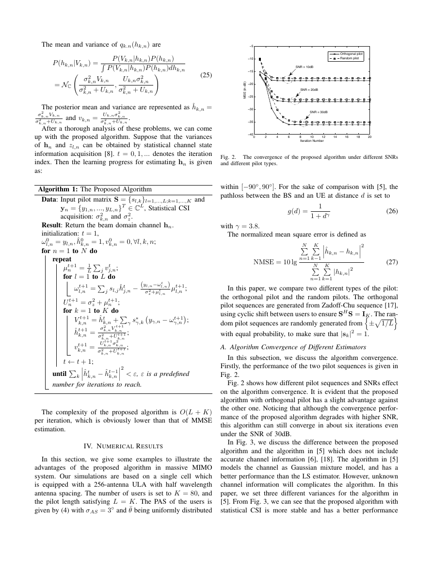Fig. 4. estimator in [5] and the proposed Bayesian estimator with statistical CSI. The MSE performance of LS estimator, MMSE estimator, the over the algorithm in [5], which may suffer a serious under- determined problem. B. MSE Performance of Different Estimators In this subsection, we provide simulation results to demon- strate the capability of the estimator. In Fig. 4, we compare six different estimators. the LS estimator achieves the MSE by MSELS = 2 z, which is the noise level. We can see that the estimator in [5] achieves better performance over the LS estimator in low SNR regions. However, it degenerates in high SNR regions. Our proposed Bayesian estimator has a significant improvement over the estimator in [5], and it approaches that of MMSE estimator. V. CONCLUSIONS In this paper, to avoid large scale matrix inversion that happen in LS or MMSE channel estimation, we investigate uplink massive MIMO channel estimation in the beam domain. Within Bayes-Optimal inference, we have proposed the new estimator with statistical CSI which can be acquired in the receiver by the detection signal. We model each channel component as a complex random variable and perform the 0510152025303540−20−18−16−14−12−10−8−6−4Iteration NumberMSE (in dB) Proposed algorithm with orthogonal pilotProposed algorithm with random pilotAlgorithm in [5] with orthogonal pilotAlgorithm in [5] with random pilot0510152025303540−50−45−40−35−30−25−20−15−10−50SNR (in dB)MSE (in dB) LS estimation with orthogonal pilotMMSE estimation with orthogonal pilotProposed algorithm with orthogonal pilotProposed algorithm with random pilotAlgorithm in [5] with random pilotAlgorithm in [5] with orthogonal pilot