Rethinking the Inception Architecture for Computer Vision.pdf

发布时间：2022-06-19 发布人：admin 分类：说明书资料大小：0.49M 资料格式：pdf 举报版权申诉

be1bca18-096f-482b-9109-2ec3b31ecc4d.pdf-第1页.png

第1页 / 共10页

be1bca18-096f-482b-9109-2ec3b31ecc4d.pdf-第2页.png

第2页 / 共10页

be1bca18-096f-482b-9109-2ec3b31ecc4d.pdf-第3页.png

第3页 / 共10页

be1bca18-096f-482b-9109-2ec3b31ecc4d.pdf-第4页.png

第4页 / 共10页

be1bca18-096f-482b-9109-2ec3b31ecc4d.pdf-第5页.png

第5页 / 共10页

be1bca18-096f-482b-9109-2ec3b31ecc4d.pdf-第6页.png

第6页 / 共10页

be1bca18-096f-482b-9109-2ec3b31ecc4d.pdf-第7页.png

第7页 / 共10页

be1bca18-096f-482b-9109-2ec3b31ecc4d.pdf-第8页.png

第8页 / 共10页

1 . Introduction

2 . General Design Principles

3 . Factorizing Convolutions with Large Filter Size

3.1 . Factorization into smaller convolutions

3.2 . Spatial Factorization into Asymmetric Convolutions

4 . Utility of Auxiliary Classifiers

5 . Efficient Grid Size Reduction

6 . Inception-v2

7 . Model Regularization via Label Smoothing

8 . Training Methodology

9 . Performance on Lower Resolution Input

10 . Experimental Results and Comparisons

11 . Conclusions

5 1 0 2 c e D 1 1 ] V C . s c [ 3 v 7 6 5 0 0 . 2 1 5 1 : v i X r a Rethinking the Inception Architecture for Computer Vision Christian Szegedy Google Inc. szegedy@google.com Vincent Vanhoucke Sergey Ioffe vanhoucke@google.com sioffe@google.com Jonathon Shlens shlens@google.com Zbigniew Wojna University College London zbigniewwojna@gmail.com Abstract Convolutional networks are at the core of most state- of-the-art computer vision solutions for a wide variety of tasks. Since 2014 very deep convolutional networks started to become mainstream, yielding substantial gains in vari- ous benchmarks. Although increased model size and com- putational cost tend to translate to immediate quality gains for most tasks (as long as enough labeled data is provided for training), computational efﬁciency and low parameter count are still enabling factors for various use cases such as mobile vision and big-data scenarios. Here we are explor- ing ways to scale up networks in ways that aim at utilizing the added computation as efﬁciently as possible by suitably factorized convolutions and aggressive regularization. We benchmark our methods on the ILSVRC 2012 classiﬁcation challenge validation set demonstrate substantial gains over the state of the art: 21.2% top-1 and 5.6% top-5 error for single frame evaluation using a network with a computa- tional cost of 5 billion multiply-adds per inference and with using less than 25 million parameters. With an ensemble of 4 models and multi-crop evaluation, we report 3.5% top-5 error and 17.3% top-1 error. 1. Introduction Since the 2012 ImageNet competition [16] winning en- try by Krizhevsky et al [9], their network “AlexNet” has been successfully applied to a larger variety of computer vision tasks, for example to object-detection [5], segmen- tation [12], human pose estimation [22], video classiﬁca- tion [8], object tracking [23], and superresolution [3]. These successes spurred a new line of research that fo- cused on ﬁnding higher performing convolutional neural networks. Starting in 2014, the quality of network architec- tures signiﬁcantly improved by utilizing deeper and wider networks. VGGNet [18] and GoogLeNet [20] yielded simi- larly high performance in the 2014 ILSVRC [16] classiﬁca- tion challenge. One interesting observation was that gains in the classiﬁcation performance tend to transfer to signiﬁ- cant quality gains in a wide variety of application domains. This means that architectural improvements in deep con- volutional architecture can be utilized for improving perfor- mance for most other computer vision tasks that are increas- ingly reliant on high quality, learned visual features. Also, improvements in the network quality resulted in new appli- cation domains for convolutional networks in cases where AlexNet features could not compete with hand engineered, crafted solutions, e.g. proposal generation in detection[4]. Although VGGNet [18] has the compelling feature of architectural simplicity, this comes at a high cost: evalu- ating the network requires a lot of computation. On the other hand, the Inception architecture of GoogLeNet [20] was also designed to perform well even under strict con- straints on memory and computational budget. For exam- ple, GoogleNet employed only 5 million parameters, which represented a 12× reduction with respect to its predeces- sor AlexNet, which used 60 million parameters. Further- more, VGGNet employed about 3x more parameters than AlexNet. The computational cost of Inception is also much lower than VGGNet or its higher performing successors [6]. This has made it feasible to utilize Inception networks in big-data scenarios[17], [13], where huge amount of data needed to be processed at reasonable cost or scenarios where memory or computational capacity is inherently limited, for example in mobile vision settings. It is certainly possible to mitigate parts of these issues by applying specialized solutions to tar- get memory use [2], [15] or by optimizing the execution of certain operations via computational tricks [10]. However, these methods add extra complexity. Furthermore, these methods could be applied to optimize the Inception archi- tecture as well, widening the efﬁciency gap again. Still, the complexity of the Inception architecture makes 1

it more difﬁcult to make changes to the network. If the ar- chitecture is scaled up naively, large parts of the computa- tional gains can be immediately lost. Also, [20] does not provide a clear description about the contributing factors that lead to the various design decisions of the GoogLeNet architecture. This makes it much harder to adapt it to new use-cases while maintaining its efﬁciency. For example, if it is deemed necessary to increase the capacity of some Inception-style model, the simple transformation of just doubling the number of all ﬁlter bank sizes will lead to a 4x increase in both computational cost and number of pa- rameters. This might prove prohibitive or unreasonable in a lot of practical scenarios, especially if the associated gains are modest. In this paper, we start with describing a few general principles and optimization ideas that that proved to be useful for scaling up convolution networks in efﬁcient ways. Although our principles are not limited to Inception- type networks, they are easier to observe in that context as the generic structure of the Inception style building blocks is ﬂexible enough to incorporate those constraints naturally. This is enabled by the generous use of dimensional reduc- tion and parallel structures of the Inception modules which allows for mitigating the impact of structural changes on nearby components. Still, one needs to be cautious about doing so, as some guiding principles should be observed to maintain high quality of the models. 2. General Design Principles Here we will describe a few design principles based on large-scale experimentation with various architectural choices with convolutional networks. At this point, the util- ity of the principles below are speculative and additional future experimental evidence will be necessary to assess their accuracy and domain of validity. Still, grave devia- tions from these principles tended to result in deterioration in the quality of the networks and ﬁxing situations where those deviations were detected resulted in improved archi- tectures in general. 1. Avoid representational bottlenecks, especially early in the network. Feed-forward networks can be repre- sented by an acyclic graph from the input layer(s) to the classiﬁer or regressor. This deﬁnes a clear direction for the information ﬂow. For any cut separating the in- puts from the outputs, one can access the amount of information passing though the cut. One should avoid bottlenecks with extreme compression. In general the representation size should gently decrease from the in- puts to the outputs before reaching the ﬁnal represen- tation used for the task at hand. Theoretically, infor- mation content can not be assessed merely by the di- mensionality of the representation as it discards impor- tant factors like correlation structure; the dimensional- ity merely provides a rough estimate of information content. 2. Higher dimensional representations are easier to pro- cess locally within a network. Increasing the activa- tions per tile in a convolutional network allows for more disentangled features. The resulting networks will train faster. 3. Spatial aggregation can be done over lower dimen- sional embeddings without much or any loss in rep- resentational power. For example, before performing a more spread out (e.g. 3 × 3) convolution, one can re- duce the dimension of the input representation before the spatial aggregation without expecting serious ad- verse effects. We hypothesize that the reason for that is the strong correlation between adjacent unit results in much less loss of information during dimension re- duction, if the outputs are used in a spatial aggrega- tion context. Given that these signals should be easily compressible, the dimension reduction even promotes faster learning. 4. Balance the width and depth of the network. Optimal performance of the network can be reached by balanc- ing the number of ﬁlters per stage and the depth of the network. Increasing both the width and the depth of the network can contribute to higher quality net- works. However, the optimal improvement for a con- stant amount of computation can be reached if both are increased in parallel. The computational budget should therefore be distributed in a balanced way between the depth and width of the network. Although these principles might make sense, it is not straightforward to use them to improve the quality of net- works out of box. The idea is to use them judiciously in ambiguous situations only. 3. Factorizing Convolutions with Large Filter Size Much of the original gains of the GoogLeNet net- work [20] arise from a very generous use of dimension re- duction. This can be viewed as a special case of factorizing convolutions in a computationally efﬁcient manner. Con- sider for example the case of a 1 × 1 convolutional layer followed by a 3 × 3 convolutional layer. In a vision net- work, it is expected that the outputs of near-by activations are highly correlated. Therefore, we can expect that their activations can be reduced before aggregation and that this should result in similarly expressive local representations. Here we explore other ways of factorizing convolutions in various settings, especially in order to increase the com- putational efﬁciency of the solution. Since Inception net- works are fully convolutional, each weight corresponds to

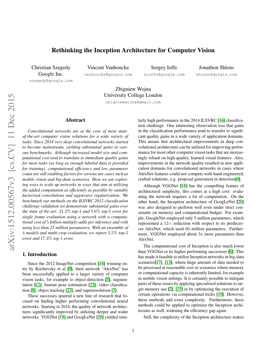
Figure 1. Mini-network replacing the 5 × 5 convolutions. one multiplication per activation. Therefore, any reduction in computational cost results in reduced number of param- eters. This means that with suitable factorization, we can end up with more disentangled parameters and therefore with faster training. Also, we can use the computational and memory savings to increase the ﬁlter-bank sizes of our network while maintaining our ability to train each model replica on a single computer. 3.1. Factorization into smaller convolutions Convolutions with larger spatial ﬁlters (e.g. 5 × 5 or 7 × 7) tend to be disproportionally expensive in terms of computation. For example, a 5 × 5 convolution with n ﬁl- ters over a grid with m ﬁlters is 25/9 = 2.78 times more computationally expensive than a 3 × 3 convolution with the same number of ﬁlters. Of course, a 5× 5 ﬁlter can cap- ture dependencies between signals between activations of units further away in the earlier layers, so a reduction of the geometric size of the ﬁlters comes at a large cost of expres- siveness. However, we can ask whether a 5× 5 convolution could be replaced by a multi-layer network with less pa- rameters with the same input size and output depth. If we zoom into the computation graph of the 5 × 5 convolution, we see that each output looks like a small fully-connected network sliding over 5× 5 tiles over its input (see Figure 1). Since we are constructing a vision network, it seems natural to exploit translation invariance again and replace the fully connected component by a two layer convolutional archi- tecture: the ﬁrst layer is a 3× 3 convolution, the second is a fully connected layer on top of the 3 × 3 output grid of the ﬁrst layer (see Figure 1). 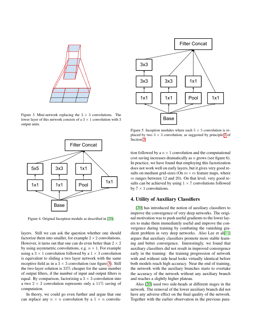Sliding this small network over the input activation grid boils down to replacing the 5 × 5 convolution with two layers of 3 × 3 convolution (compare Figure 4 with 5). This setup clearly reduces the parameter count by shar- ing the weights between adjacent tiles. 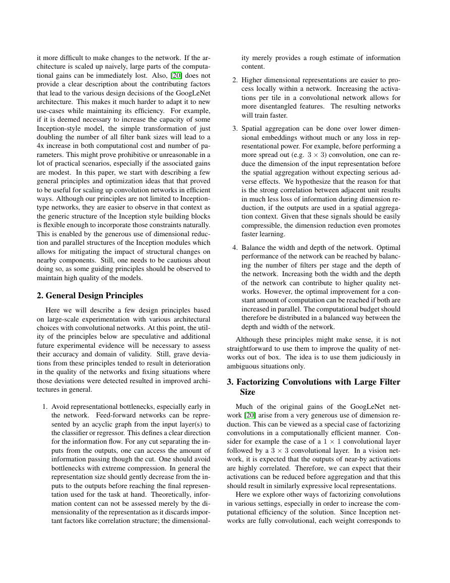To analyze the ex- Figure 2. One of several control experiments between two Incep- tion models, one of them uses factorization into linear + ReLU layers, the other uses two ReLU layers. After 3.86 million opera- tions, the former settles at 76.2%, while the latter reaches 77.2% top-1 Accuracy on the validation set. √ pected computational cost savings, we will make a few sim- plifying assumptions that apply for the typical situations: We can assume that n = αm, that is that we want to change the number of activations/unit by a constant alpha factor. Since the 5 × 5 convolution is aggregating, α is typically slightly larger than one (around 1.5 in the case of GoogLeNet). Having a two layer replacement for the 5 × 5 layer, it seems reasonable to reach this expansion in two steps: increasing the number of ﬁlters by α in both steps. In order to simplify our estimate by choosing α = 1 (no expansion), If we would naivly slide a network without reusing the computation between neighboring grid tiles, we would increase the computational cost. sliding this network can be represented by two 3× 3 convolutional layers which reuses the activations between adjacent tiles. This way, we 25 × reduction of computation, resulting end up with a net 9+9 in a relative gain of 28% by this factorization. The exact same saving holds for the parameter count as each parame- ter is used exactly once in the computation of the activation of each unit. Still, this setup raises two general questions: Does this replacement result in any loss of expressiveness? If our main goal is to factorize the linear part of the compu- tation, would it not suggest to keep linear activations in the ﬁrst layer? We have ran several control experiments (for ex- ample see ﬁgure 2) and using linear activation was always inferior to using rectiﬁed linear units in all stages of the fac- torization. We attribute this gain to the enhanced space of variations that the network can learn especially if we batch- normalize [7] the output activations. One can see similar effects when using linear activations for the dimension re- duction components. 3.2. Spatial Factorization into Asymmetric Convo- lutions The above results suggest that convolutions with ﬁlters larger 3 × 3 a might not be generally useful as they can always be reduced into a sequence of 3 × 3 convolutional 00.511.522.533.54x 10600.10.20.30.40.50.60.70.8IterationTop−1 AccuracyFactorization with Linear vs ReLU activation ReLULinear

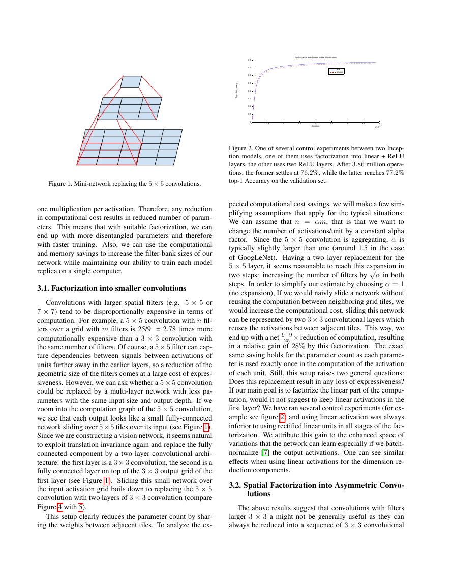
Figure 3. Mini-network replacing the 3 × 3 convolutions. The lower layer of this network consists of a 3 × 1 convolution with 3 output units. Figure 4. Original Inception module as described in [20]. layers. Still we can ask the question whether one should factorize them into smaller, for example 2× 2 convolutions. However, it turns out that one can do even better than 2 × 2 by using asymmetric convolutions, e.g. n × 1. For example using a 3 × 1 convolution followed by a 1 × 3 convolution is equivalent to sliding a two layer network with the same receptive ﬁeld as in a 3 × 3 convolution (see ﬁgure 3). Still the two-layer solution is 33% cheaper for the same number of output ﬁlters, if the number of input and output ﬁlters is equal. By comparison, factorizing a 3 × 3 convolution into a two 2 × 2 convolution represents only a 11% saving of computation. In theory, we could go even further and argue that one can replace any n × n convolution by a 1 × n convolu- Figure 5. Inception modules where each 5 × 5 convolution is re- placed by two 3 × 3 convolution, as suggested by principle 3 of Section 2. tion followed by a n× 1 convolution and the computational cost saving increases dramatically as n grows (see ﬁgure 6). In practice, we have found that employing this factorization does not work well on early layers, but it gives very good re- sults on medium grid-sizes (On m× m feature maps, where m ranges between 12 and 20). On that level, very good re- sults can be achieved by using 1 × 7 convolutions followed by 7 × 1 convolutions. 4. Utility of Auxiliary Classiﬁers [20] has introduced the notion of auxiliary classiﬁers to improve the convergence of very deep networks. The origi- nal motivation was to push useful gradients to the lower lay- ers to make them immediately useful and improve the con- vergence during training by combating the vanishing gra- dient problem in very deep networks. Also Lee et al[11] argues that auxiliary classiﬁers promote more stable learn- ing and better convergence. Interestingly, we found that auxiliary classiﬁers did not result in improved convergence early in the training: the training progression of network with and without side head looks virtually identical before both models reach high accuracy. Near the end of training, the network with the auxiliary branches starts to overtake the accuracy of the network without any auxiliary branch and reaches a slightly higher plateau. Also [20] used two side-heads at different stages in the network. The removal of the lower auxiliary branch did not have any adverse effect on the ﬁnal quality of the network. Together with the earlier observation in the previous para- 1x1 1x1 5x5 3x3 Pool 1x1 BaseFilter Concat1x1 1x1 1x1 3x3 3x3 Pool 1x1 BaseFilter Concat3x3 1x1

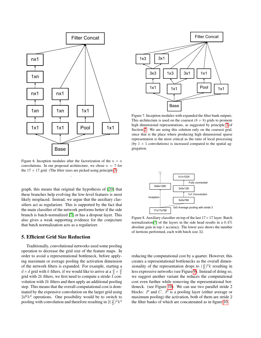
Figure 7. Inception modules with expanded the ﬁlter bank outputs. This architecture is used on the coarsest (8 × 8) grids to promote high dimensional representations, as suggested by principle 2 of Section 2. We are using this solution only on the coarsest grid, since that is the place where producing high dimensional sparse representation is the most critical as the ratio of local processing (by 1 × 1 convolutions) is increased compared to the spatial ag- gregation. 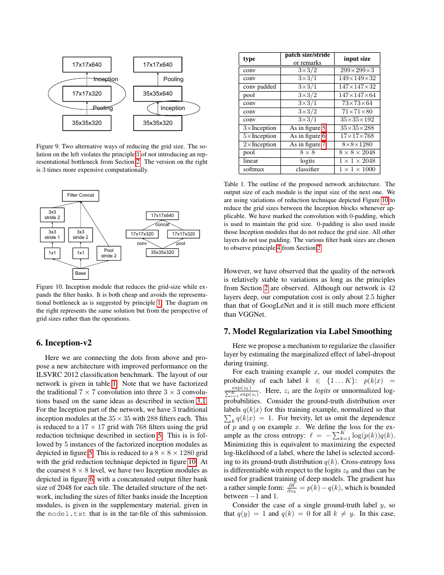Figure 8. Auxiliary classiﬁer on top of the last 17×17 layer. Batch normalization[7] of the layers in the side head results in a 0.4% absolute gain in top-1 accuracy. The lower axis shows the number of itertions performed, each with batch size 32. reducing the computational cost by a quarter. However, this creates a representational bottlenecks as the overall dimen- sionality of the representation drops to ( d 2 )2k resulting in less expressive networks (see Figure 9). Instead of doing so, we suggest another variant the reduces the computational cost even further while removing the representational bot- tleneck. (see Figure 10). We can use two parallel stride 2 blocks: P and C. P is a pooling layer (either average or maximum pooling) the activation, both of them are stride 2 the ﬁlter banks of which are concatenated as in ﬁgure 10. Figure 6. Inception modules after the factorization of the n × n convolutions. In our proposed architecture, we chose n = 7 for the 17 × 17 grid. (The ﬁlter sizes are picked using principle 3) . graph, this means that original the hypothesis of [20] that these branches help evolving the low-level features is most likely misplaced. Instead, we argue that the auxiliary clas- siﬁers act as regularizer. This is supported by the fact that the main classiﬁer of the network performs better if the side branch is batch-normalized [7] or has a dropout layer. This also gives a weak supporting evidence for the conjecture that batch normalization acts as a regularizer. 5. Efﬁcient Grid Size Reduction Traditionally, convolutional networks used some pooling operation to decrease the grid size of the feature maps. In order to avoid a representational bottleneck, before apply- ing maximum or average pooling the activation dimension of the network ﬁlters is expanded. For example, starting a d× d grid with k ﬁlters, if we would like to arrive at a d 2 × d 2 grid with 2k ﬁlters, we ﬁrst need to compute a stride-1 con- volution with 2k ﬁlters and then apply an additional pooling step. This means that the overall computational cost is dom- inated by the expensive convolution on the larger grid using 2d2k2 operations. One possibility would be to switch to pooling with convolution and therefore resulting in 2( d 2 )2k2 1x1 1x1 1xn Pool 1x1 BaseFilter Concatnx1 1xn nx1 1xn nx1 1x1 1x1 1x1 3x3 Pool 1x1 BaseFilter Concat1x3 1x3 1x1 3x1 3x1 17x17x7685x5x7688x8x1280Inception5x5x1281x1x10245x5 Average pooling with stride 31x1 Convolution Fully connected...

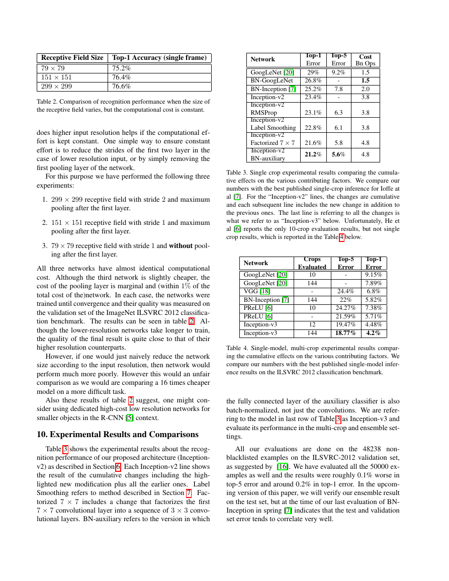
type conv conv conv padded pool conv conv conv 3×Inception 5×Inception 2×Inception pool linear softmax patch size/stride or remarks 3×3/2 3×3/1 3×3/1 3×3/2 3×3/1 3×3/2 3×3/1 As in ﬁgure 5 As in ﬁgure 6 As in ﬁgure 7 8 × 8 logits classiﬁer input size 299×299×3 149×149×32 147×147×32 147×147×64 73×73×64 71×71×80 35×35×192 35×35×288 17×17×768 8×8×1280 8 × 8 × 2048 1 × 1 × 2048 1 × 1 × 1000 Table 1. The outline of the proposed network architecture. The output size of each module is the input size of the next one. We are using variations of reduction technique depicted Figure 10 to reduce the grid sizes between the Inception blocks whenever ap- plicable. We have marked the convolution with 0-padding, which is used to maintain the grid size. 0-padding is also used inside those Inception modules that do not reduce the grid size. All other layers do not use padding. The various ﬁlter bank sizes are chosen to observe principle 4 from Section 2. However, we have observed that the quality of the network is relatively stable to variations as long as the principles from Section 2 are observed. Although our network is 42 layers deep, our computation cost is only about 2.5 higher than that of GoogLeNet and it is still much more efﬁcient than VGGNet. exp(zk) 7. Model Regularization via Label Smoothing Here we propose a mechanism to regularize the classiﬁer layer by estimating the marginalized effect of label-dropout during training. For each training example x, our model computes the probability of each label k ∈ {1 . . . K}: p(k|x) = K i=1 exp(zi). Here, zi are the logits or unnormalized log- probabilities. Consider the ground-truth distribution over labels q(k|x) for this training example, normalized so that k q(k|x) = 1. For brevity, let us omit the dependence ample as the cross entropy: = −K of p and q on example x. We deﬁne the loss for the ex- k=1 log(p(k))q(k). Minimizing this is equivalent to maximizing the expected log-likelihood of a label, where the label is selected accord- ing to its ground-truth distribution q(k). Cross-entropy loss is differentiable with respect to the logits zk and thus can be used for gradient training of deep models. The gradient has = p(k)− q(k), which is bounded a rather simple form: ∂ between −1 and 1. ∂zk Consider the case of a single ground-truth label y, so that q(y) = 1 and q(k) = 0 for all k = y. 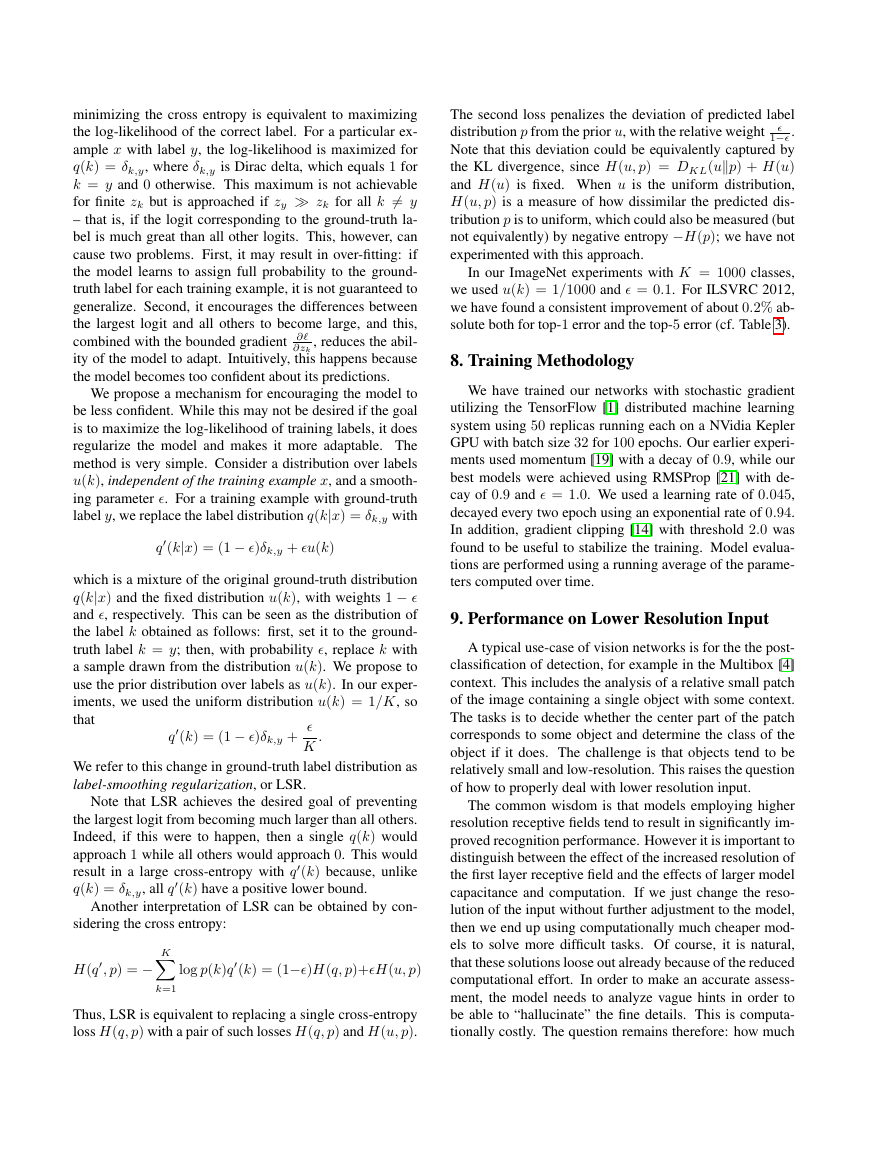In this case, Figure 9. Two alternative ways of reducing the grid size. The so- lution on the left violates the principle 1 of not introducing an rep- resentational bottleneck from Section 2. The version on the right is 3 times more expensive computationally. Figure 10. Inception module that reduces the grid-size while ex- pands the ﬁlter banks. It is both cheap and avoids the representa- tional bottleneck as is suggested by principle 1. The diagram on the right represents the same solution but from the perspective of grid sizes rather than the operations. 6. Inception-v2 Here we are connecting the dots from above and pro- pose a new architecture with improved performance on the ILSVRC 2012 classiﬁcation benchmark. The layout of our network is given in table 1. Note that we have factorized the traditional 7 × 7 convolution into three 3 × 3 convolu- tions based on the same ideas as described in section 3.1. For the Inception part of the network, we have 3 traditional inception modules at the 35× 35 with 288 ﬁlters each. This is reduced to a 17 × 17 grid with 768 ﬁlters using the grid reduction technique described in section 5. This is is fol- lowed by 5 instances of the factorized inception modules as depicted in ﬁgure 5. This is reduced to a 8 × 8 × 1280 grid with the grid reduction technique depicted in ﬁgure 10. At the coarsest 8 × 8 level, we have two Inception modules as depicted in ﬁgure 6, with a concatenated output ﬁlter bank size of 2048 for each tile. The detailed structure of the net- work, including the sizes of ﬁlter banks inside the Inception modules, is given in the supplementary material, given in the model.txt that is in the tar-ﬁle of this submission. 35x35x32017x17x32017x17x640PoolingInception35x35x32035x35x64017x17x640InceptionPoolingPoolstride 2 BaseFilter Concat1x1 3x3stride 2 3x3stride 1 1x1 3x3stride 2 35x35x32017x17x32017x17x32017x17x640poolconvconcat

minimizing the cross entropy is equivalent to maximizing the log-likelihood of the correct label. For a particular ex- ample x with label y, the log-likelihood is maximized for q(k) = δk,y, where δk,y is Dirac delta, which equals 1 for k = y and 0 otherwise. This maximum is not achievable for ﬁnite zk but is approached if zy zk for all k = y – that is, if the logit corresponding to the ground-truth la- bel is much great than all other logits. This, however, can cause two problems. First, it may result in over-ﬁtting: if the model learns to assign full probability to the ground- truth label for each training example, it is not guaranteed to generalize. Second, it encourages the differences between the largest logit and all others to become large, and this, , reduces the abil- combined with the bounded gradient ∂ ∂zk ity of the model to adapt. Intuitively, this happens because the model becomes too conﬁdent about its predictions. We propose a mechanism for encouraging the model to be less conﬁdent. While this may not be desired if the goal is to maximize the log-likelihood of training labels, it does regularize the model and makes it more adaptable. The method is very simple. Consider a distribution over labels u(k), independent of the training example x, and a smooth- ing parameter . For a training example with ground-truth label y, we replace the label distribution q(k|x) = δk,y with q(k|x) = (1 − )δk,y + u(k) which is a mixture of the original ground-truth distribution q(k|x) and the ﬁxed distribution u(k), with weights 1 − and , respectively. This can be seen as the distribution of the label k obtained as follows: ﬁrst, set it to the ground- truth label k = y; then, with probability , replace k with a sample drawn from the distribution u(k). We propose to use the prior distribution over labels as u(k). In our exper- iments, we used the uniform distribution u(k) = 1/K, so that q(k) = (1 − )δk,y + K . We refer to this change in ground-truth label distribution as label-smoothing regularization, or LSR. Note that LSR achieves the desired goal of preventing the largest logit from becoming much larger than all others. Indeed, if this were to happen, then a single q(k) would approach 1 while all others would approach 0. This would result in a large cross-entropy with q(k) because, unlike q(k) = δk,y, all q(k) have a positive lower bound. Another interpretation of LSR can be obtained by con- sidering the cross entropy: H(q, p) = − K log p(k)q(k) = (1−)H(q, p)+H(u, p) k=1 Thus, LSR is equivalent to replacing a single cross-entropy loss H(q, p) with a pair of such losses H(q, p) and H(u, p). The second loss penalizes the deviation of predicted label distribution p from the prior u, with the relative weight 1−. Note that this deviation could be equivalently captured by the KL divergence, since H(u, p) = DKL(up) + H(u) and H(u) is ﬁxed. When u is the uniform distribution, H(u, p) is a measure of how dissimilar the predicted dis- tribution p is to uniform, which could also be measured (but not equivalently) by negative entropy −H(p); we have not experimented with this approach. In our ImageNet experiments with K = 1000 classes, we used u(k) = 1/1000 and = 0.1. For ILSVRC 2012, we have found a consistent improvement of about 0.2% ab- solute both for top-1 error and the top-5 error (cf. Table 3). 8. Training Methodology We have trained our networks with stochastic gradient utilizing the TensorFlow [1] distributed machine learning system using 50 replicas running each on a NVidia Kepler GPU with batch size 32 for 100 epochs. Our earlier experi- ments used momentum [19] with a decay of 0.9, while our best models were achieved using RMSProp [21] with de- cay of 0.9 and = 1.0. We used a learning rate of 0.045, decayed every two epoch using an exponential rate of 0.94. In addition, gradient clipping [14] with threshold 2.0 was found to be useful to stabilize the training. Model evalua- tions are performed using a running average of the parame- ters computed over time. 9. Performance on Lower Resolution Input A typical use-case of vision networks is for the the post- classiﬁcation of detection, for example in the Multibox [4] context. This includes the analysis of a relative small patch of the image containing a single object with some context. The tasks is to decide whether the center part of the patch corresponds to some object and determine the class of the object if it does. The challenge is that objects tend to be relatively small and low-resolution. This raises the question of how to properly deal with lower resolution input. The common wisdom is that models employing higher resolution receptive ﬁelds tend to result in signiﬁcantly im- proved recognition performance. However it is important to distinguish between the effect of the increased resolution of the ﬁrst layer receptive ﬁeld and the effects of larger model capacitance and computation. If we just change the reso- lution of the input without further adjustment to the model, then we end up using computationally much cheaper mod- els to solve more difﬁcult tasks. Of course, it is natural, that these solutions loose out already because of the reduced computational effort. In order to make an accurate assess- ment, the model needs to analyze vague hints in order to be able to “hallucinate” the ﬁne details. This is computa- tionally costly. The question remains therefore: how much

Receptive Field Size Top-1 Accuracy (single frame) 79 × 79 151 × 151 299 × 299 75.2% 76.4% 76.6% Table 2. Comparison of recognition performance when the size of the receptive ﬁeld varies, but the computational cost is constant. does higher input resolution helps if the computational ef- fort is kept constant. One simple way to ensure constant effort is to reduce the strides of the ﬁrst two layer in the case of lower resolution input, or by simply removing the ﬁrst pooling layer of the network. For this purpose we have performed the following three experiments: 1. 299 × 299 receptive ﬁeld with stride 2 and maximum pooling after the ﬁrst layer. 2. 151 × 151 receptive ﬁeld with stride 1 and maximum pooling after the ﬁrst layer. 3. 79× 79 receptive ﬁeld with stride 1 and without pool- ing after the ﬁrst layer. All three networks have almost identical computational cost. Although the third network is slightly cheaper, the cost of the pooling layer is marginal and (within 1% of the total cost of the)network. In each case, the networks were trained until convergence and their quality was measured on the validation set of the ImageNet ILSVRC 2012 classiﬁca- tion benchmark. The results can be seen in table 2. Al- though the lower-resolution networks take longer to train, the quality of the ﬁnal result is quite close to that of their higher resolution counterparts. However, if one would just naively reduce the network size according to the input resolution, then network would perform much more poorly. However this would an unfair comparison as we would are comparing a 16 times cheaper model on a more difﬁcult task. Also these results of table 2 suggest, one might con- sider using dedicated high-cost low resolution networks for smaller objects in the R-CNN [5] context. 10. Experimental Results and Comparisons Table 3 shows the experimental results about the recog- nition performance of our proposed architecture (Inception- v2) as described in Section 6. Each Inception-v2 line shows the result of the cumulative changes including the high- lighted new modiﬁcation plus all the earlier ones. Label Smoothing refers to method described in Section 7. Fac- torized 7 × 7 includes a change that factorizes the ﬁrst 7 × 7 convolutional layer into a sequence of 3 × 3 convo- lutional layers. BN-auxiliary refers to the version in which Network GoogLeNet [20] BN-GoogLeNet BN-Inception [7] Inception-v2 Inception-v2 RMSProp Inception-v2 Label Smoothing Inception-v2 Factorized 7 × 7 Inception-v2 BN-auxiliary Top-1 Error 29% 26.8% 25.2% 23.4% 23.1% 22.8% Top-5 Error 9.2% - 7.8 - 6.3 6.1 21.6% 5.8 21.2% 5.6% Cost Bn Ops 1.5 1.5 2.0 3.8 3.8 3.8 4.8 4.8 Table 3. Single crop experimental results comparing the cumula- tive effects on the various contributing factors. We compare our numbers with the best published single-crop inference for Ioffe at al [7]. For the “Inception-v2” lines, the changes are cumulative and each subsequent line includes the new change in addition to the previous ones. The last line is referring to all the changes is what we refer to as “Inception-v3” below. Unfortunately, He et al [6] reports the only 10-crop evaluation results, but not single crop results, which is reported in the Table 4 below. Network GoogLeNet [20] GoogLeNet [20] VGG [18] BN-Inception [7] PReLU [6] PReLU [6] Inception-v3 Inception-v3 Crops Evaluated 10 144 - 144 10 - 12 144 - - Top-5 Error Top-1 Error 9.15% 7.89% 6.8% 5.82% 24.27% 7.38% 21.59% 5.71% 19.47% 4.48% 18.77% 4.2% 24.4% 22% Table 4. Single-model, multi-crop experimental results compar- ing the cumulative effects on the various contributing factors. We compare our numbers with the best published single-model infer- ence results on the ILSVRC 2012 classiﬁcation benchmark. the fully connected layer of the auxiliary classiﬁer is also batch-normalized, not just the convolutions. We are refer- ring to the model in last row of Table 3 as Inception-v3 and evaluate its performance in the multi-crop and ensemble set- tings. All our evaluations are done on the 48238 non- blacklisted examples on the ILSVRC-2012 validation set, as suggested by [16]. We have evaluated all the 50000 ex- amples as well and the results were roughly 0.1% worse in top-5 error and around 0.2% in top-1 error. In the upcom- ing version of this paper, we will verify our ensemble result on the test set, but at the time of our last evaluation of BN- Inception in spring [7] indicates that the test and validation set error tends to correlate very well.

分享到：

赞收藏

资料库

Rethinking the Inception Architecture for Computer Vision.pdf

相关推荐

人工智能

热门标签

最新资料