RVM Explained.pdf-资料库

f09e2680-582e-46b7-bc23-06d885cfd0d6.pdf-第1页.png

第1页 / 共10页

f09e2680-582e-46b7-bc23-06d885cfd0d6.pdf-第2页.png

第2页 / 共10页

f09e2680-582e-46b7-bc23-06d885cfd0d6.pdf-第3页.png

第3页 / 共10页

f09e2680-582e-46b7-bc23-06d885cfd0d6.pdf-第4页.png

第4页 / 共10页

f09e2680-582e-46b7-bc23-06d885cfd0d6.pdf-第5页.png

第5页 / 共10页

f09e2680-582e-46b7-bc23-06d885cfd0d6.pdf-第6页.png

第6页 / 共10页

f09e2680-582e-46b7-bc23-06d885cfd0d6.pdf-第7页.png

第7页 / 共10页

f09e2680-582e-46b7-bc23-06d885cfd0d6.pdf-第8页.png

第8页 / 共10页

October 19, 2010 Relevance Vector Machines Explained Tristan Fletcher www.cs.ucl.ac.uk/staﬀ/T.Fletcher/

Introduction This document has been written in an attempt to make Tipping’s [1] Rele- vance Vector Machines (RVM) as simple to understand as possible for those with minimal experience of Machine Learning. It assumes knowledge of probability in the areas of Bayes’ theorem and Gaussian distributions in- cluding marginal and conditional Gaussian distributions. It also assumes familiarity with matrix diﬀerentiation, the vector representation of regres- sion and kernel (basis) functions. These latter two areas are brieﬂy covered in the author’s similar paper on Support Vector Machines which can be found through the URL on the coverpage. The document has been split into two main sections. The ﬁrst introduces the problem that needs to be solved, namely maximising the posterior probabil- ity of regression target values over some hyperparameters. It then proceeds to derive the equations required to do this. Aside from the areas mentioned above where knowledge is assumed, every mathematical step is gone through. It is therefore hoped that there is no ambiguity over any of the details in this explanation, though this does make the description a little cumbersome. The second section therefore explains from an algorithmic viewpoint the it- erations that would be required to actually apply the technique. Aside from Tipping [1], the majority of this document is based on work by MacKay [2], [3], [4], [5] and Bishop [6]. Notation With the view of making this description as explicit (in the mathematical sense) as possible, it is worth introducing some of the notation that will be used: • P (A|B, C) is the probability of A given B and C. Note that using this notation, diﬀerent representations of the parameters will not alter this probability, e.g. P (A|B) ≡ P (A|B−1). Furthermore, for the sake of simplicity, occasionally some of the elements in the probabilistic notation will be omitted where they are not relevant, e.g. P (A|B) ≡ P (A|B, C, D etc). • X ∼ N (µ, σ2) is used to signify that X is normally distributed with mean µ and variance σ2. • Bold font is used to represent vectors and matrices. 1

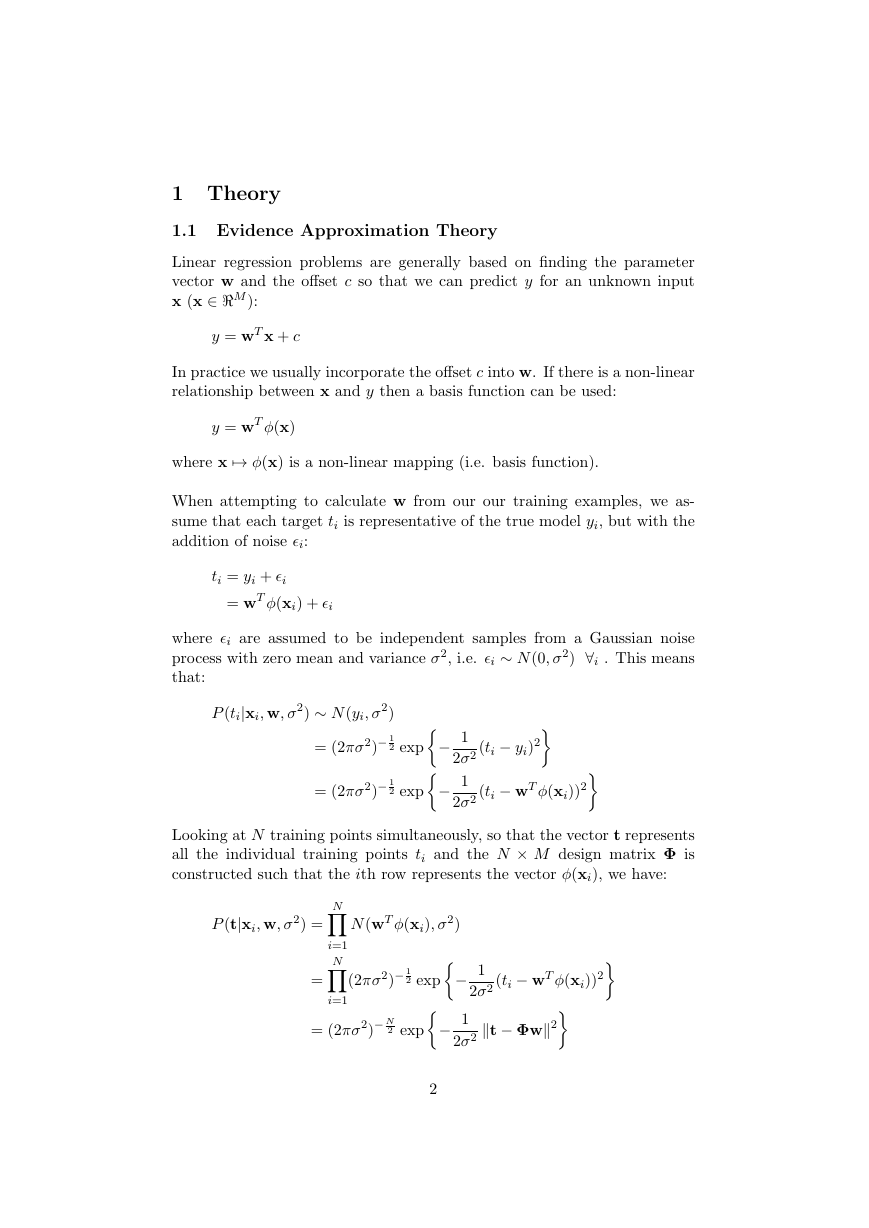
1 Theory 1.1 Evidence Approximation Theory Linear regression problems are generally based on ﬁnding the parameter vector w and the oﬀset c so that we can predict y for an unknown input x (x ∈ M ): y = wT x + c In practice we usually incorporate the oﬀset c into w. If there is a non-linear relationship between x and y then a basis function can be used: y = wT φ(x) where x → φ(x) is a non-linear mapping (i.e. basis function). When attempting to calculate w from our our training examples, we as- sume that each target ti is representative of the true model yi, but with the addition of noise i: ti = yi + i = wT φ(xi) + i where i are assumed to be independent samples from a Gaussian noise process with zero mean and variance σ2, i.e. i ∼ N (0, σ2) ∀i . This means that: P (ti|xi, w, σ2) ∼ N (yi, σ2) = (2πσ2)− 1 2 exp = (2πσ2)− 1 2 exp − 1 2σ2 (ti − yi)2 − 1 2σ2 (ti − wT φ(xi))2 Looking at N training points simultaneously, so that the vector t represents all the individual training points ti and the N × M design matrix Φ is constructed such that the ith row represents the vector φ(xi), we have: N N i=1 P (t|xi, w, σ2) = = N (wT φ(xi), σ2) (2πσ2)− 1 2 exp i=1 = (2πσ2)− N 2 exp − 1 2σ2 (ti − wT φ(xi))2 − 1 2σ2 t − Φw2 2

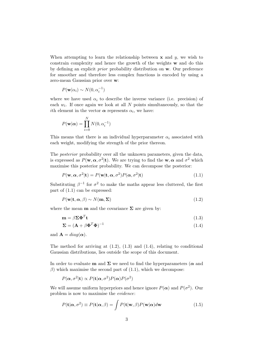
When attempting to learn the relationship between x and y, we wish to constrain complexity and hence the growth of the weights w and do this by deﬁning an explicit prior probability distribution on w. Our preference for smoother and therefore less complex functions is encoded by using a zero-mean Gaussian prior over w: P (w|αi) ∼ N (0, α−1 i ) where we have used αi to describe the inverse variance (i.e. precision) of each wi. If once again we look at all N points simultaneously, so that the ith element in the vector α represents αi, we have: N P (w|α) = N (0, α−1 i ) i=0 This means that there is an individual hyperparameter αi associated with each weight, modifying the strength of the prior thereon. The posterior probability over all the unknown parameters, given the data, is expressed as P (w, α, σ2|t). We are trying to ﬁnd the w, α and σ2 which maximise this posterior probability. We can decompose the posterior: P (w, α, σ2|t) = P (w|t, α, σ2)P (α, σ2|t) (1.1) Substituting β−1 for σ2 to make the maths appear less cluttered, the ﬁrst part of (1.1) can be expressed: P (w|t, α, β) ∼ N (m, Σ) (1.2) where the mean m and the covariance Σ are given by: m = βΣΦT t Σ = (A + βΦT Φ)−1 and A = diag(α). (1.3) (1.4) The method for arriving at (1.2), (1.3) and (1.4), relating to conditional Gaussian distributions, lies outside the scope of this document. In order to evaluate m and Σ we need to ﬁnd the hyperparameters (α and β) which maximise the second part of (1.1), which we decompose: P (α, σ2|t) ∝ P (t|α, σ2)P (α)P (σ2) We will assume uniform hyperpriors and hence ignore P (α) and P (σ2). Our problem is now to maximise the evidence: P (t|α, σ2) ≡ P (t|α, β) = P (t|w, β)P (w|α)dw (1.5) 3

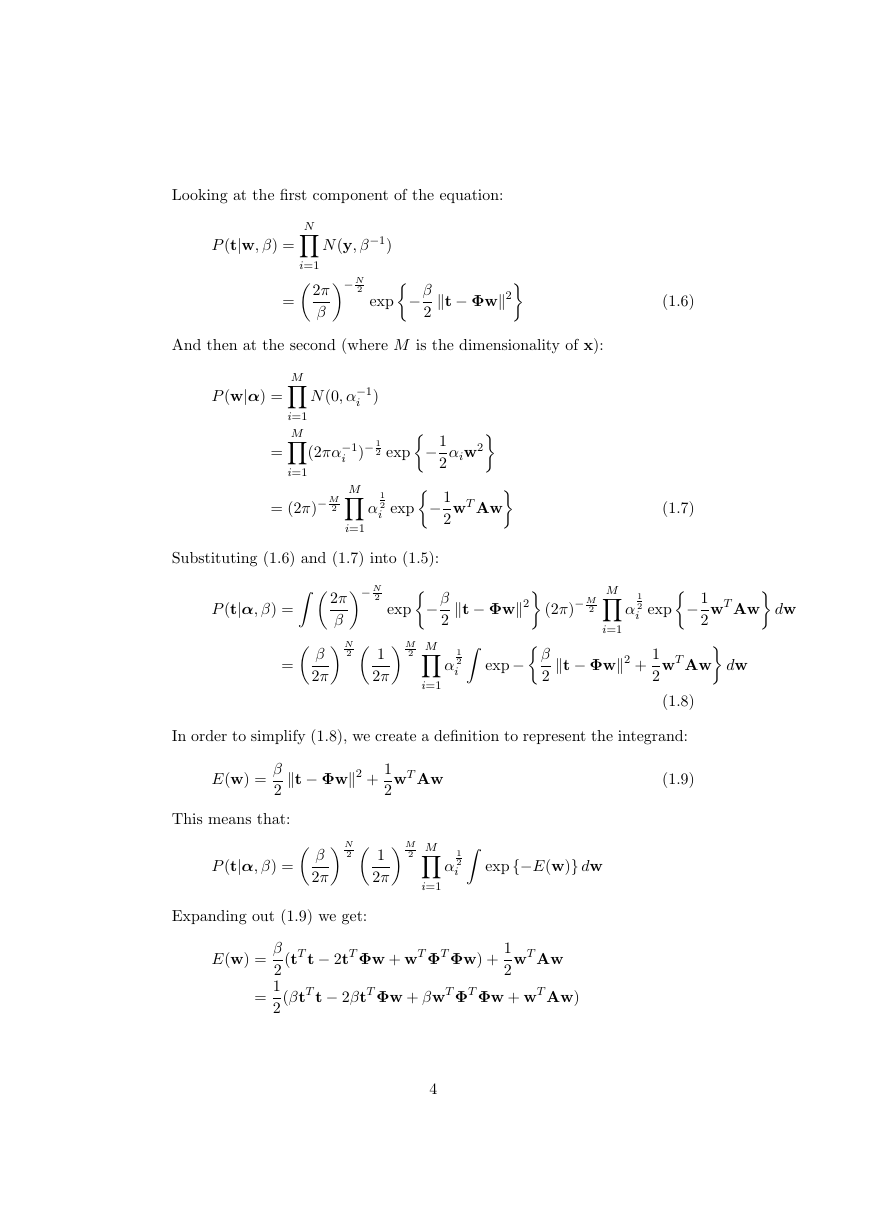
Looking at the ﬁrst component of the equation: P (t|w, β) = = N (y, β−1) − N 2 exp t − Φw2 − β 2 (1.6) And then at the second (where M is the dimensionality of x): N 2π i=1 β M M i=1 P (w|α) = = N (0, α−1 i ) αiw2 − 1 2 − 1 2 α i exp wT Aw (2πα−1 2 exp i )− 1 M 1 2 i=1 i=1 = (2π)− M 2 Substituting (1.6) and (1.7) into (1.5): − N 2π N β 2 1 β 2 M M 2 − β 2 exp 2π 2π i=1 β 2 t − Φw2 (2π)− M 2 1 2 i α exp− P (t|α, β) = = (1.7) − 1 2 1 2 i exp α M i=1 dw wT Aw dw t − Φw2 + wT Aw 1 2 (1.8) In order to simplify (1.8), we create a deﬁnition to represent the integrand: E(w) = β 2 t − Φw2 + 1 2 wT Aw (1.9) This means that: P (t|α, β) = β 2π 2 1 N M 2 2π M i=1 1 2 i α exp{−E(w)} dw Expanding out (1.9) we get: E(w) = = β 2 1 2 (tT t − 2tT Φw + wT ΦT Φw) + (βtT t − 2βtT Φw + βwT ΦT Φw + wT Aw) wT Aw 1 2 4

Substituting in (1.4) and then using I = Σ−1Σ: E(w) = = 1 2 1 2 (βtT t − 2βtT Φw + wT Σ−1w) (βtT t − 2βtT ΦΣ−1Σw + wT Σ−1w) Substituting in (1.3): E(w) = 1 2 (βtT t − 2mT Σ−1w + wT Σ−1w + mT Σ−1m − mT Σ−1m) = E(t) + 1 2 (w − m)T Σ−1(w − m) where E(t) = (βtT t − mT Σ−1m) 1 2 Our integrand from (1.8) now becomes: exp{−E(w)} dw = exp{−E(t)} (2π) M 2 |Σ| 1 2 Substituting this back in, gives us: β 2 1 N M 2 2π 2π M i=1 1 2 i exp{−E(t)} (2π) α M 2 |Σ| 1 2 P (t|α, β) = This is known as our marginal likelihood and taking logs, gives us our log marginal likelihood : M i=1 ln P (t|α, β) = N 2 ln β − E(t) − 1 2 ln|Σ| − N 2 ln(2π) + 1 2 ln αi (1.10) It is this equation we need to maximise with respect to α and β, a process known as the evidence approximation procedure. 1.2 Evidence Approximation Procedure In order to maximise our log marginal likelihood, we start by taking deriva- tives of (1.10) with respect to αi and setting these to zero: ln P (t|α, β) = d dαi 1 2αi ⇒ αi = Σii − 1 − 1 2 2 1 − αiΣii m2 i = 0 m2 i 5

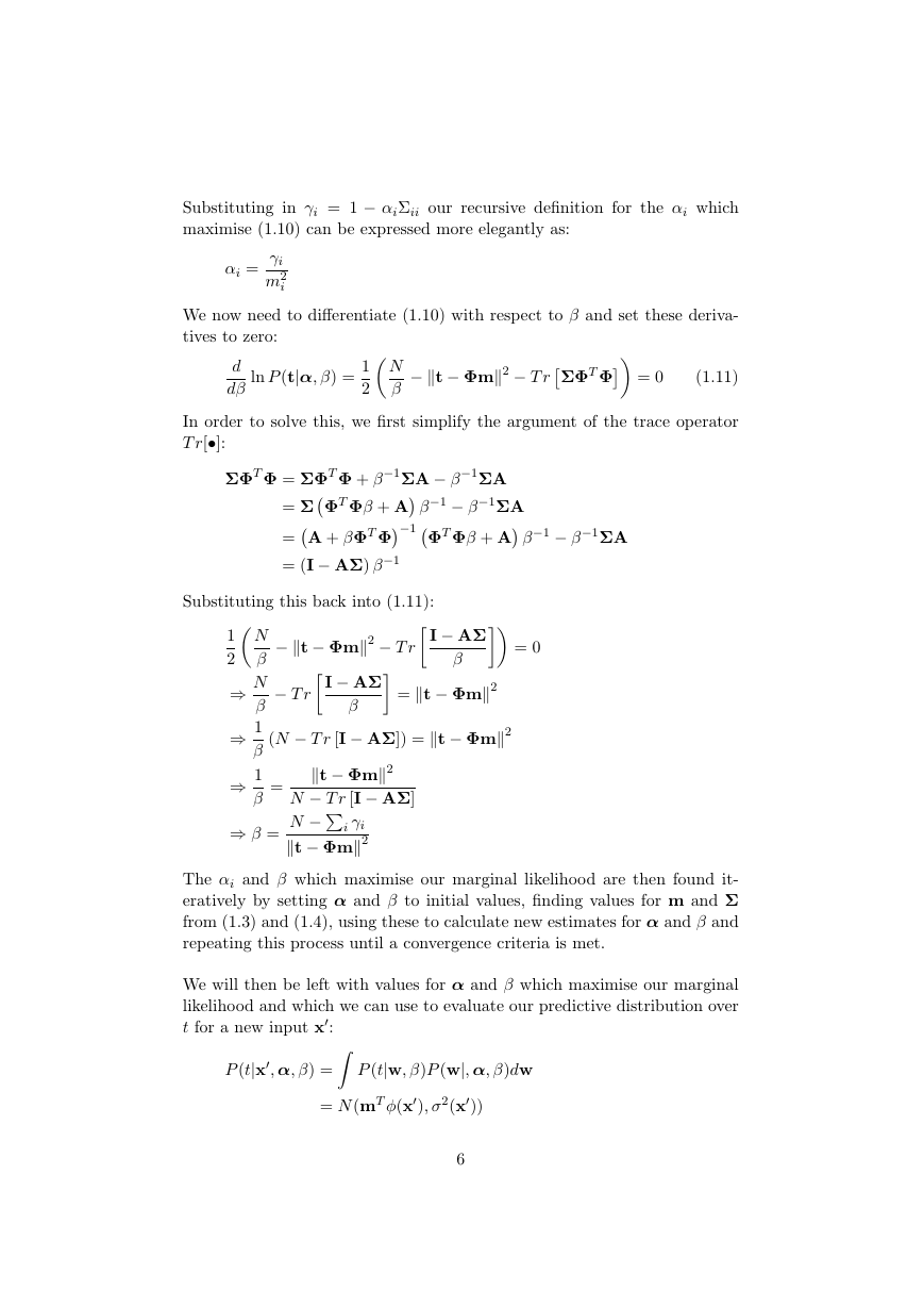
Substituting in γi = 1 − αiΣii our recursive deﬁnition for the αi which maximise (1.10) can be expressed more elegantly as: αi = γi m2 i We now need to diﬀerentiate (1.10) with respect to β and set these deriva- tives to zero: N β − t − Φm2 − T rΣΦT Φ ln P (t|α, β) = d dβ 1 2 = 0 (1.11) In order to solve this, we ﬁrst simplify the argument of the trace operator T r[•]: ΣΦT Φ = ΣΦT Φ + β−1ΣA − β−1ΣA = ΣΦT Φβ + A β−1 − β−1ΣA =A + βΦT Φ−1ΦT Φβ + A β−1 − β−1ΣA = (I − AΣ) β−1 Substituting this back into (1.11): I − AΣ = 0 β = t − Φm2 − t − Φm2 − T r I − AΣ − T r β (N − T r [I − AΣ]) = t − Φm2 N 1 2 β ⇒ N β ⇒ 1 β ⇒ 1 β = N − T r [I − AΣ] t − Φm2 N − i γi t − Φm2 ⇒ β = The αi and β which maximise our marginal likelihood are then found it- eratively by setting α and β to initial values, ﬁnding values for m and Σ from (1.3) and (1.4), using these to calculate new estimates for α and β and repeating this process until a convergence criteria is met. We will then be left with values for α and β which maximise our marginal likelihood and which we can use to evaluate our predictive distribution over t for a new input x: P (t|x, α, β) = P (t|w, β)P (w|, α, β)dw = N (mT φ(x), σ2(x)) 6

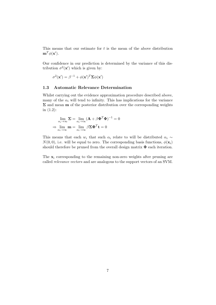
This means that our estimate for t is the mean of the above distribution mT φ(x). Our conﬁdence in our prediction is determined by the variance of this dis- tribution σ2(x) which is given by: σ2(x) = β−1 + φ(x)T Σφ(x) 1.3 Automatic Relevance Determination Whilst carrying out the evidence approximation procedure described above, many of the αi will tend to inﬁnity. This has implications for the variance Σ and mean m of the posterior distribution over the corresponding weights in (1.2): lim αi→∞ Σ = lim ⇒ lim αi→∞ m = lim αi→∞(A + βΦT Φ)−1 = 0 αi→∞ βΣΦT t = 0 This means that each wi that such αi relate to will be distributed αi ∼ N (0, 0), i.e. will be equal to zero. The corresponding basis functions, φ(xi) should therefore be pruned from the overall design matrix Φ each iteration. The xi corresponding to the remaining non-zero weights after pruning are called relevance vectors and are analogous to the support vectors of an SVM. 7

资料库

RVM Explained.pdf

相关推荐

课程资源

热门标签

最新资料