[2015][40]Bayesian estimation of the DINA model with Gibbs sampl....pdf

发布时间：2022-06-02 发布人：admin 分类：说明书资料大小：1.43M 资料格式：pdf 举报版权申诉

maerdym-12563104-16359648044581624020.pdf-第1页.png

第1页 / 共23页

maerdym-12563104-16359648044581624020.pdf-第2页.png

第2页 / 共23页

maerdym-12563104-16359648044581624020.pdf-第3页.png

第3页 / 共23页

maerdym-12563104-16359648044581624020.pdf-第4页.png

第4页 / 共23页

maerdym-12563104-16359648044581624020.pdf-第5页.png

第5页 / 共23页

maerdym-12563104-16359648044581624020.pdf-第6页.png

第6页 / 共23页

maerdym-12563104-16359648044581624020.pdf-第7页.png

第7页 / 共23页

maerdym-12563104-16359648044581624020.pdf-第8页.png

第8页 / 共23页

文本预览

JOURNAL OF EDUCATIONAL AND BEHAVIORAL STATISTICS OnlineFirst, published on August 10, 2015 as doi:10.3102/1076998615595403 Journal of Educational and Behavioral Statistics Vol. XX, No. X, pp. 1–23 DOI: 10.3102/1076998615595403 # 2015 AERA. http://jebs.aera.net Bayesian Estimation of the DINA Model With Gibbs Sampling Steven Andrew Culpepper University of Illinois at Urbana-Champaign A Bayesian model formulation of the deterministic inputs, noisy ‘‘and’’ gate (DINA) model is presented. Gibbs sampling is employed to simulate from the joint posterior distribution of item guessing and slipping parameters, subject attribute parameters, and latent class probabilities. The procedure extends concepts in Be´guin and Glas, Culpepper, and Sahu for estimating the guessing and slipping parameters in the three- and four-parameter normal-ogive models. The ability of the model to recover parameters is demonstrated in a simulation study. The technique is applied to a mental rotation test. The algorithm and vignettes are freely available to researchers as the ‘‘dina’’ R package. Keywords: cognitive diagnosis; bayesian statistics; markov chain monte carlo; spatial cognition Introduction Cognitive diagnosis models (CDMs) remain an important methodology for diagnosing student skill acquisition. A variety of CDMs have been developed. In particular, existing CDMs include the deterministic inputs, noisy ‘‘and’’ gate (DINA) model (de la Torre, 2009a; de la Torre & Douglas, 2004, 2008; Doignon & Falmagne, 1999; Haertel, 1989; Junker & Sijtsma, 2001; Macready & Dayton, 1977), the noisy inputs, deterministic, ‘‘and’’ gate (NIDA) model (Maris, 1999), the deterministic input, noisy ‘‘or’’ gate (DINO) model (Templin & Henson, 2006b), the reduced reparameterized unified model (RUM; Roussos, DiBello, et al., 2007), the generalized DINA (de la Torre, 2011), the log-linear CDM (Henson, Templin, & Willse, 2009), and the general diagnostic model (von Davier, 2008). The aforementioned models differ in complexity, and prior research demonstrated how models such as the DINA, NIDA, and DINO can be estimated in more generalized frameworks (e.g., see de la Torre, 2011; von Davier, 2014). The interpretability of the DINA model makes it a popular CDM (de la Torre, 2009a; von Davier, 2014), and the purpose of this article is to introduce a Bayesian formulation for estimating the DINA model parameters with Gibbs sampling. This article includes five sections. The first section introduces the DINA model and discusses benefits of the proposed Bayesian formulation in the context 1 Downloaded from http://jebs.aera.net at CMU Libraries - library.cmich.edu on December 8, 2015

Bayesian Estimation of the DINA of prior research. The second section presents the Bayesian model formulation and full conditional distributions that are used to estimate person (i.e., latent skill/attribute profiles) and item parameters (i.e., slipping and guessing) using Markov Chain Monte Carlo (MCMC) with Gibbs sampling. The third section reports results from a simulation study on the accuracy of recovering the model parameters. The fourth section presents an application of the model using responses to a mental rotation test (Guay, 1976; Yoon, 2011). The final section includes discussion, future research directions, and concluding remarks. The DINA Model Overview Throughout this article, let i ¼ 1; . . . ; N index individuals, j ¼ 1; . . . ; J index items, k ¼ 1; . . . ; K index skills, and c ¼ 1; . . . ; C index latent classes. CDMs assume that a set of K known skills underlie each item. The skills needed to succeed on each item are collected into a J K matrix Q, which is a structure matrix with elements that are akin to factor loadings relating skills to items. How- ever, one exception is that the elements of Q are either 0 or 1 (i.e., qjk 2 f0; 1g) depending upon whether skill k is needed for success on item j. That is, qjk equals 1 if skill k is needed to correctly answer item j and 0 otherwise. Let j ¼ ðqj1; . . . ; qjKÞ be the j th row of Q ¼ ðq1; . . . ; qJÞ0 , which indicates the 0 q requisite skills for item j. The DINA model posits that individual test takers are classified into latent classes based upon mastery and nonmastery of the K skills. Let aik equal 1 if individual i has mastered skill k and zero otherwise. Furthermore, let the K dimensional latent attribute profile of binary indicators for individual i be αi ¼ ðai1; :::; aiKÞ0 . Given the categorical nature of the latent classes, αi can equal one of C¼ 2K attribute profiles. It will be useful subsequently to define αc ¼ ðac1; . . . ; acKÞ0 as the attribute profile for members of class c such that ack is 1 if members of class c possess skill k and zero otherwise. The DINA model is a conjunctive model, which implies that students need to correctly answer item j without guessing. We all of the skills in qj let the vector of ideal responses for student i be η jqjÞ, where I denotes the indicator function. Zij ¼ ∏K Notice that Zij is 1 if student i has the requisite skills to answer item j and 0 if the student is missing at least one skill. The probability of individual i’s success on item j for the DINA model is a function of individual latent class membership (i.e., αi) and item parameters, i ¼ ðZi1; . . . ; ZiJÞ0 ik ¼ Iðα0 iqj ¼ q with k¼1aqjk 0 ( Pðyij ¼ 1jαi; ΩjÞ ¼ 2 gj; Zij ¼ ∏K 1 sj; Zij ¼ ∏K k¼1aqjk k¼1aqjk ik ¼ 0 ik ¼ 1 ; (1) Downloaded from http://jebs.aera.net at CMU Libraries - library.cmich.edu on December 8, 2015

Culpepper where Ωj ¼ ðgj; sjÞ is a row vector of gj ¼ Pðyij ¼ 1jZij ¼ 0Þ is the probability of correctly guessing item j for students sj ¼ Pðyij ¼ 0jZij ¼ 1Þ is the probability of ‘‘slipping,’’ which is defined as the who do not have the requisite skills needed for item parameters. By definition, In contrast, item j. chance that students who have the required skills to answer item j record an incorrect response. The DINA item response function can be used to construct a likelihood of observing a sample of item responses. Let yi ¼ ðyi1; . . . ; yiJÞ0 denote a J dimen- sional vector of item responses for individual i, where yij is coded as 1 for a cor- rect response and 0 for an incorrect response. Let Ω ¼ ðΩ1; . . . ; ΩJÞ be a row let vector of slipping and guessing parameters for J items. Furthermore, Pjc ¼ Pðy ¼ 1jαc; ΩjÞ be the probability that members of class c correctly answer item j and note that αi ¼ αc implies that individual i is in attribute class c. Assuming that item responses are conditionally independent given αi, the probability of observing yi given membership in class c (i.e., αi ¼ αc) is, pðyijαi ¼ αc; ΩÞ ¼ ∏J j¼1 yij jc ð1 PjcÞ1yij : P (2) Let c ¼ pðαcÞ be the marginal probability of belonging to class c in the pop- ulation and define π ¼ ð1; . . . ; CÞ0 as a C dimensional vector of class member- ship probabilities. The Law of Total Probability implies that the probability of X observing yi given item parameters Ω and latent class probabilities π is given by, The likelihood of observing a sample of N responses to J items is given by, pðyaijΩ; πÞ ¼ pðyjΩ; πÞ ¼ ∏N i¼1 c¼1 C c¼1 cpðyijαi ¼ αc; ΩÞ: X cpðyijαi ¼ αac; ΩÞ; C (3) (4) where y ¼ ðy1; . . . ; yNÞ0 is an N J matrix of observed responses. In Bayesian formulations, the primary focus is on the parameter posterior dis- tribution, which for the DINA model is, pðΩ; πjyÞ / pðyj ; πÞpðΩÞpðπÞ; (5) where pðΩÞ is a prior distribution for item parameters and pðπÞ is a prior distri- bution for latent class probabilities. Maris (1999) noted the intractable nature of the CDM parameter posterior distributions and alluded to how Monte Carlo procedures could be used to estimate posterior distributions. Accordingly, subse- quent research considered MCMC procedures for estimating posterior distribu- tions of CDM parameters (de la Torre & Douglas, 2004; Hartz, 2002; Henson et al., 2009; Templin, 2004). Roussos, Templin, and Henson (2007) provide an 3 Downloaded from http://jebs.aera.net at CMU Libraries - library.cmich.edu on December 8, 2015

Bayesian Estimation of the DINA overview of estimation methods (both Bayesian and non-Bayesian) prior researchers have employed to estimate CDM parameters. Furthermore, prior research discussed how applied researchers can estimate CDMs with standard statistical software (de la Torre, 2009b; Henson et al., 2009; Rupp, 2009; Rupp, Templin, & Henson, 2010). Benefits of the Proposed Bayesian Formulation The Bayesian model formulation for the DINA CDM developed in this article offers several benefits to the existing procedures. First, the model formulation yields analytically tractable full conditional distributions for the person and item parameters that enable the use of Gibbs sampling for efficient computations. Prior applications of the DINA model and other CDMs employed Metropolis- Hastings (MH) sampling to estimate model parameters, which require tuning of proposal distribution parameters for Ω and π. Consequently, one limitation with using MH sampling is that researchers need to tune proposal parameters each time a new data set is analyzed. More specifically, researchers who use MH sampling to estimate DINA model parameters need to choose proposal para- meters to ensure no more than 50% of candidates are accepted. Specifying tuning parameters may require only a few attempts for a given data set, but the process could become tedious if the goal is to disseminate software for widespread use by applied researchers who have less experience with MH sampling. In contrast, the procedures discussed subsequently employ Gibbs sampling from parameter full conditional distributions and can be easily implemented without manual tuning. As another example, consider the additional requirements needed to employ MH sampling in a simulation study similar to the one reported subsequently. After developing estimation code and deciding upon simulation conditions, it would be necessary to select proposal parameters used to sample candidates for Ω and π. Proposal parameters must be tuned using trial and error, where a col- lection of chains are run with different proposal parameter values to ensure 25–50% of candidates are accepted. It would be necessary to apply the tuning process for all conditions of the simulation study, which, depending upon the number of conditions, could require considerable effort to verify and catalogue proposal distribution parameter values. In contrast, employing the Gibbs sampler developed in this article would only require decisions about prior parameters. The procedure introduced subsequently employs uninformative uniform priors for Ω and π, so the developed algorithm can be immediately applied. Second, the proposed formulation is advantageous to prior Gibbs samplers. For instance, prior CDM research employed Gibbs sampling to estimate the reparameterized DINA model using OpenBUGS (DeCarlo, 2012) and the higher order DINA (HO-DINA) model (de la Torre & Douglas, 2004) using WinBUGS (Li, 2008). However, one disadvantage is that OpenBUGS and WinBUGS do not explicitly impose the monotonicity restriction for the DINA model that 4 Downloaded from http://jebs.aera.net at CMU Libraries - library.cmich.edu on December 8, 2015

Culpepper 0 gj þ sj < 1 for all items (Junker & Sijtsma, 2001). One consequence is that prior Gibbs samplers did not strictly enforce the identifiability condition, which could impact convergence in some applications. The model discussed subse- quently extends the Bayesian formulation of the three-parameter normal-ogive (3PNO) model of Be´guin and Glass (2001) and Sahu (2002) and the four- parameter model of Culpepper (in press) to explicitly enforce the monotonicity requirement. Accordingly, the developed strategy could be extended to other CDMs that include guessing and slipping parameters such as the NIDA, DINO, and RUM. Third, one documented advantage of using Gibbs sampling is improved mix- ing of the chain in comparison to procedures based upon acceptance/rejection sampling such as MH sampling. That is, prior research suggests that MH sam- pling mixes best (i.e., the posterior distribution is efficiently explored) if candi- dates are accepted between 25% and 50% of the iterations (e.g., see chapter 6 of Robert & Casella, 2009). Accordingly, MH sampling may contribute to slower mixing among posterior samples, given that posterior samples change in less than half the total iterations. In contrast, the Gibbs sampler has the potential to improve mixing by sampling values from full conditional distributions. How- ever, as noted by an anonymous reviewer, Gibbs sampling does not guarantee faster mixing for all models and parameters (e.g., see Cowles, 1996, for discus- sion regarding threshold parameters in polytomous normal-ogive models). The Monte Carlo evidence given subsequently suggests that the proposed MCMC algorithm converges to the parameter posterior distribution within 350 to 750 iterations. In contrast, prior research that employed Bayesian estimation (DeCarlo, 2012; Henson et al., 2009; Li, 2008) reported requiring a burn-in between 1,000 and 5,000 iterations to achieve convergence. Fourth, as discussed subsequently, students’ latent attribute profiles are mod- eled using a general categorical prior. One advantage is that specifying a catego- rical prior provides a natural approach for computing the probability of skill acquisition and classifying students into latent classes (Huebner & Wang, 2011). That is, the posterior distribution for each student’s skill distribution can be sum- marized to show the probability of membership in the various latent classes. Fifth, the developed algorithm is made freely available to researchers as the ‘‘dina’’ R package. The Gibbs sampler was written in Cþþ and provides an effi- cient approach for estimating model parameters. In fact, the developed R pack- age includes documentation and vignettes to instruct applied researchers. Bayesian Estimation of the DINA Model This section presents a Bayesian formulation for the DINA model. The first section presents the model and describes the priors and the second section pre- sents the full conditional distributions for implementation in an MCMC Gibbs sampler. 5 Downloaded from http://jebs.aera.net at CMU Libraries - library.cmich.edu on December 8, 2015

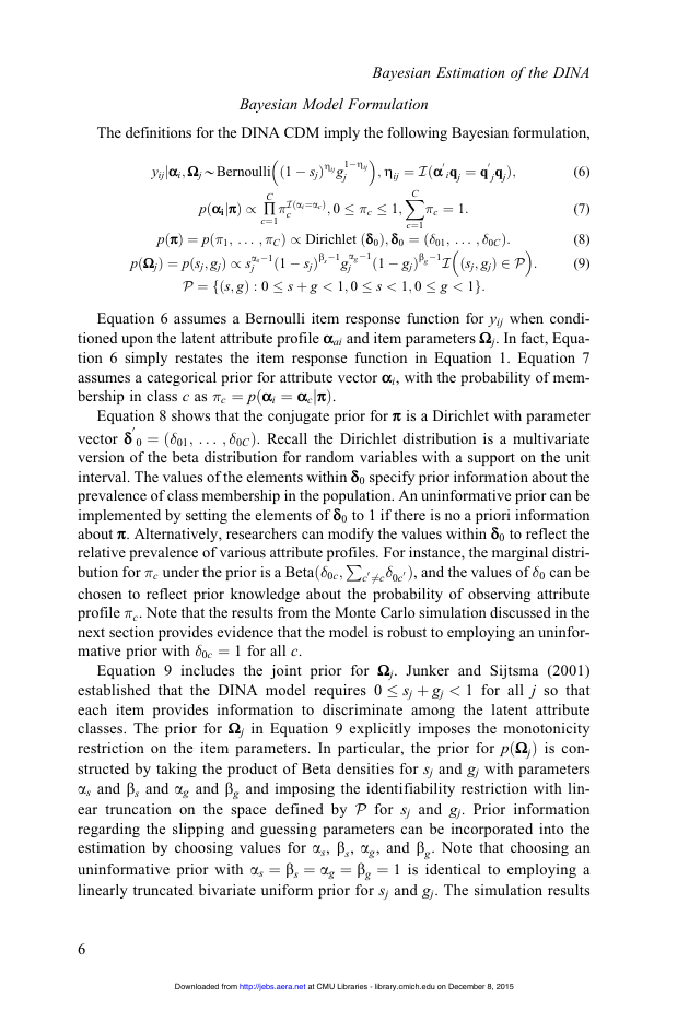
Bayesian Estimation of the DINA The definitions for the DINA CDM imply the following Bayesian formulation, Bayesian Model Formulation 1Zij j yijjαi; Ωj*Bernoulli pðαijπÞ / ∏C c¼1 ð1 sjÞZij g Iðai¼acÞ c ; 0 c 1; 0 jqjÞ; X iqj ¼ q ; Zij ¼ Iðα0 c ¼ 1: c¼1 C pðπÞ ¼ pð1; . . . ; CÞ / Dirichlet ðδ0Þ; δ0 ¼ ð01; . . . ; 0CÞ: pðΩjÞ ¼ pðsj; gjÞ / s as1 j ð1 sjÞbs1g ag1 j ð1 gjÞbg1I ðsj; gjÞ 2 P P ¼ fðs; gÞ : 0 s þ g < 1; 0 s < 1; 0 g < 1g: (6) (7) (8) (9) : P Equation 6 assumes a Bernoulli item response function for yij when condi- tioned upon the latent attribute profile αai and item parameters Ωj. In fact, Equa- tion 6 simply restates the item response function in Equation 1. Equation 7 assumes a categorical prior for attribute vector αi, with the probability of mem- bership in class c as c ¼ pðαi ¼ αcjπÞ. Equation 8 shows that the conjugate prior for π is a Dirichlet with parameter 0 ¼ ð01; . . . ; 0CÞ. Recall the Dirichlet distribution is a multivariate vector δ0 version of the beta distribution for random variables with a support on the unit interval. The values of the elements within δ0 specify prior information about the prevalence of class membership in the population. An uninformative prior can be implemented by setting the elements of δ0 to 1 if there is no a priori information about π. Alternatively, researchers can modify the values within δ0 to reflect the relative prevalence of various attribute profiles. For instance, the marginal distri- bution for c under the prior is a Betað0c; 0Þ, and the values of 0 can be chosen to reflect prior knowledge about the probability of observing attribute profile c. Note that the results from the Monte Carlo simulation discussed in the next section provides evidence that the model is robust to employing an uninfor- mative prior with 0c ¼ 1 for all c. Equation 9 includes the joint prior for Ωj. Junker and Sijtsma (2001) established that the DINA model requires 0 sj þ gj < 1 for all j so that each item provides information to discriminate among the latent attribute classes. The prior for Ωj in Equation 9 explicitly imposes the monotonicity restriction on the item parameters. In particular, the prior for pðΩjÞ is con- structed by taking the product of Beta densities for sj and gj with parameters as and bs and ag and bg and imposing the identifiability restriction with lin- ear truncation on the space defined by P for sj and gj. Prior information regarding the slipping and guessing parameters can be incorporated into the estimation by choosing values for as, bs, ag, and bg. Note that choosing an uninformative prior with as ¼ bs ¼ ag ¼ bg ¼ 1 is identical to employing a linearly truncated bivariate uniform prior for sj and gj. The simulation results 06¼c0c c 6 Downloaded from http://jebs.aera.net at CMU Libraries - library.cmich.edu on December 8, 2015

Culpepper discussed in the next section support the use of uninformative priors for the slipping and guessing parameters. Full Conditional Distributions The full conditional distributions for αi, π, and Ωj are, pðαijyi; π; ΩÞ ¼ ∏C c¼1 πjα1; . . . ; αN / DirichletðN ic ~ Iðαi¼αcÞ X ; ~ ic ¼ pðαi ¼ αcjyi; π; ΩÞ: X þ δ0Þ: Iðαi ¼ αCÞ N Iðai ¼ a1Þ; . . . ; N0 ¼ ðN 1; . . . ;N CÞ ¼ (10) (11) N i¼1 i¼1 ð1 gjÞb~ s 1I ðsj; gjÞ 2 P pðΩjjyj;Z1j; . . . ;ZNjÞ / s a~ j s 1 g 1 a~ j s 1g ð1 sjÞb~ s ¼ T j Sj þ bs X X g ¼ N T j Gj þ bg a~ a~ s ¼ Sj þ as;b~ g ¼ Gj þ ag;b~ X Zij; Sj ¼ N T j ¼ i¼1 N Zij; Gj ¼ N ð1 ZijÞ: (12) ijyij¼0 ijyij¼1 Equation 10 shows that the full conditional for αi is a categorical distribution with the probability of membership in category c as ~ ic. Specifically, Bayes’s theorem implies that the probability that student i belongs to class c given yi, Ω, and π is, ~ ic ¼ pðαi ¼ αcjyi; π; ΩÞ ¼ (13) X pðyijαi ¼ αc; ΩÞc C c¼1 cpðyijαi ¼ αc; ΩÞ : ~ The full conditional for αi is a categorical distribution with probabilities i1; . . . ; ~ Equation 11 reports the full conditional distribution for π. Specifically, the full iC. conditional distribution for π can be derived as, pðπjα1; . . . ; αNÞ / pðα1; . . . ; αNjπÞpðπÞ ¼ ∏N i¼1 cþ0c N c ¼ ∏N i¼1 c ¼ ∏C 0c c¼1 Iðai¼acÞ c ∏C c¼1 ∏C c¼1 pðπÞ pðαijπÞ : (14) Equation 14 shows that the full conditional for π is the product of the catego- rical prior for αi, and the Dirichlet prior for π. Let the number of students within the C latent classes for a given MCMC iteration be denoted by the vector N0 ¼ ðN i¼1Iðαi ¼ αcÞ is the number of subjects CÞ such that N 1; . . . ; N within attribute class c. Accordingly, the full conditional for the latent class prob- þ δ0Þ. abilities in Equation 14 is DirichletðN P c ¼ N 7 Downloaded from http://jebs.aera.net at CMU Libraries - library.cmich.edu on December 8, 2015

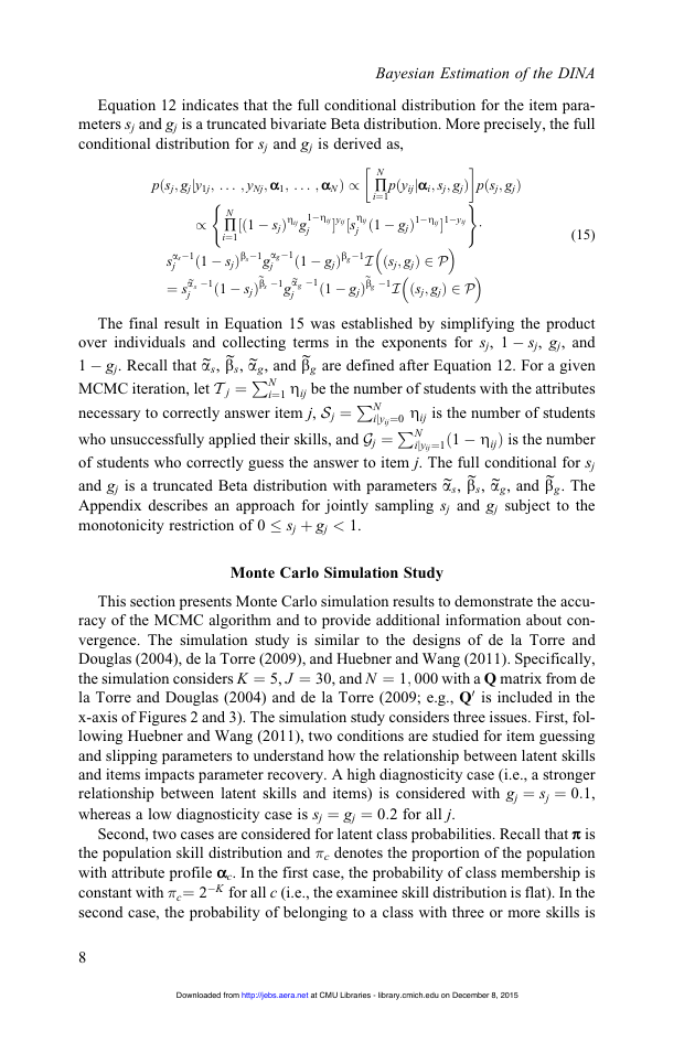
Bayesian Estimation of the DINA Equation 12 indicates that the full conditional distribution for the item para- meters sj and gj is a truncated bivariate Beta distribution. More precisely, the full conditional distribution for sj and gj is derived as, ) pðyijjαi; sj; gjÞ pðsj; gjÞ pðsj; gjjy1j; . . . ; yNj; α1; . . . ; αNÞ / ∏N i¼1 j ð1 gjÞ1Zij1yij ½ð1 sjÞZij g yij½s ( 1Zij Zij j (15) ∏N i¼1 / ð1 sjÞbs1g s 1 ð1 sjÞb~ as1 s j ¼ s a~ j ag1 j s 1g ð1 gjÞbg1I g 1 ð1 gjÞb~ a~ j ðsj; gjÞ 2 P g 1I ðsj; gjÞ 2 P N P The final result in Equation 15 was established by simplifying the product P over individuals and collecting terms in the exponents for sj, 1 sj, gj, and 1 gj. Recall that a~ g, and b~ s, b~ s, a~ g are defined after Equation 12. For a given MCMC iteration, let T j ¼ i¼1 Zij be the number of students with the attributes necessary to correctly answer item j, Sj ¼ ijyij¼0 Zij is the number of students who unsuccessfully applied their skills, and Gj ¼ ijyij¼1ð1 ZijÞ is the number of students who correctly guess the answer to item j. The full conditional for sj and gj is a truncated Beta distribution with parameters a~ g. The Appendix describes an approach for jointly sampling sj and gj subject to the monotonicity restriction of 0 sj þ gj < 1. g, and b~ P s, b~ s, a~ N N Monte Carlo Simulation Study This section presents Monte Carlo simulation results to demonstrate the accu- racy of the MCMC algorithm and to provide additional information about con- vergence. The simulation study is similar to the designs of de la Torre and Douglas (2004), de la Torre (2009), and Huebner and Wang (2011). 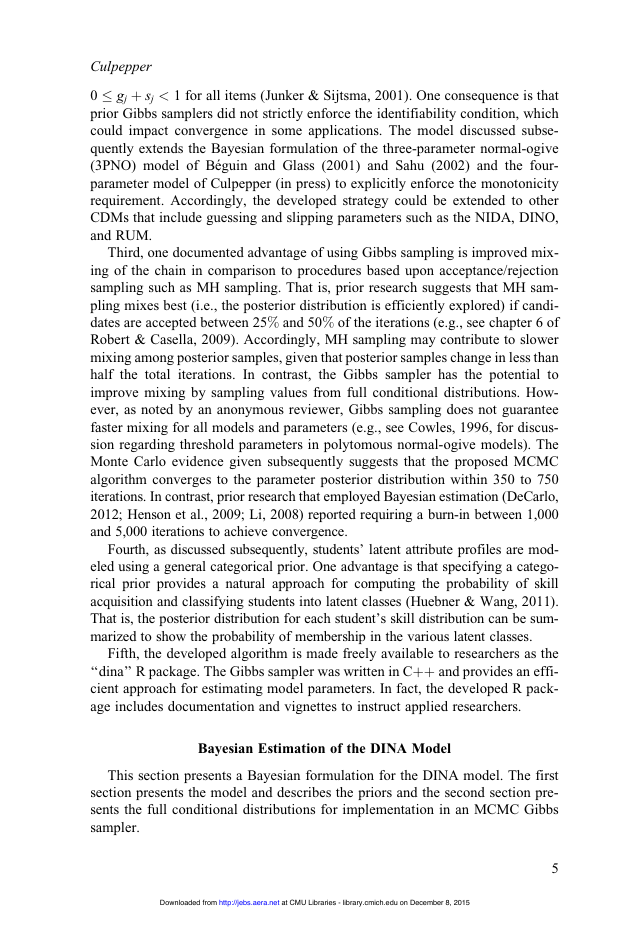Specifically, the simulation considers K ¼ 5, J ¼ 30, and N ¼ 1; 000 with a Q matrix from de la Torre and Douglas (2004) and de la Torre (2009; e.g., Q0 is included in the x-axis of Figures 2 and 3). The simulation study considers three issues. First, fol- lowing Huebner and Wang (2011), two conditions are studied for item guessing and slipping parameters to understand how the relationship between latent skills and items impacts parameter recovery. A high diagnosticity case (i.e., a stronger relationship between latent skills and items) is considered with gj ¼ sj ¼ 0:1, whereas a low diagnosticity case is sj ¼ gj ¼ 0:2 for all j. Second, two cases are considered for latent class probabilities. Recall that π is the population skill distribution and c denotes the proportion of the population with attribute profile α c. In the first case, the probability of class membership is constant with c¼ 2K for all c (i.e., the examinee skill distribution is flat). In the second case, the probability of belonging to a class with three or more skills is 8 Downloaded from http://jebs.aera.net at CMU Libraries - library.cmich.edu on December 8, 2015

分享到：

赞收藏

资料库

[2015][40]Bayesian estimation of the DINA model with Gibbs sampl....pdf

相关推荐

行业

热门标签

最新资料