s
s
a
l
c
e
l
c
i
t
r
a
L
O
P
I
5
.
0
v
1
0
/
7
0
/
4
1
0
2
Published in Image Processing On Line on 2011–02–24.
Submitted on 2011–00–00, accepted on 2011–00–00.
ISSN 2105–1232 c 2011 IPOL & the authors CC–BY–NC–SA
This article is available online with supplementary materials,
software, datasets and online demo at
http://dx.doi.org/10.5201/ipol.2011.my-asift
ASIFT: An Algorithm for Fully Affine Invariant Comparison
Guoshen Yu1, Jean-Michel Morel2
1 CMAP, ´Ecole Polytechnique, France (yu@cmap.polytechnique.fr)
2 CMLA, ENS Cachan, France (moreljeanmichel@gmail.com)
Abstract
If a physical object has a smooth or piecewise smooth boundary, its images obtained by cameras
in varying positions undergo smooth apparent deformations. These deformations are locally
well approximated by affine transforms of the image plane.
In consequence the solid object
recognition problem has often been led back to the computation of affine invariant image local
features. The similarity invariance (invariance to translation, rotation, and zoom) is dealt with
rigorously by the SIFT method The method illustrated and demonstrated in this work, Affine-
SIFT (ASIFT), simulates a set of sample views of the initial images, obtainable by varying the
two camera axis orientation parameters, namely the latitude and the longitude angles, which
are not treated by the SIFT method. Then it applies the SIFT method itself to all images thus
generated. Thus, ASIFT covers effectively all six parameters of the affine transform.
The source code (ANSI C), its documentation, and the online demo are accessible at the IPOL
web page of this article1.
Source Code
Keywords: SIFT; affine invariant matching
1 Overview
If a physical object has a smooth or piecewise smooth boundary, its images obtained by cameras
in varying positions undergo smooth apparent deformations. These deformations are locally well
approximated by affine transforms of the image plane.
In consequence the solid object recognition problem has often been led back to the computation
of affine invariant image local features. Such invariant features could be obtained by normalization
methods, but no fully affine normalization method exists for the time being. Yet as shown in [7]
the similarity invariance (invariance to translation, rotation, and zoom) is dealt with rigorously by
the SIFT method [1]. By simulating on both images zooms out and by normalizing translation and
rotation, the SIFT method succeeds in being fully invariant to four out of the six parameters of an
affine transform.
1http://dx.doi.org/10.5201/ipol.2011.my-asift
Guoshen Yu, Jean-Michel Morel, ASIFT: An Algorithm for Fully Affine Invariant Comparison, Image Processing On Line, 1 (2011), pp. 1–28.
http://dx.doi.org/10.5201/ipol.2011.my-asift
�
Guoshen Yu, Jean-Michel Morel
The method illustrated and demonstrated in this work, Affine-SIFT (ASIFT), simulates a set of
sample views of the initial images, obtainable by varying the two camera axis orientation parameters,
namely the latitude and the longitude angles, which are not treated by the SIFT method. Then it
applies the SIFT method itself to all images thus generated. Thus, ASIFT covers effectively all six
parameters of the affine transform. The method is mathematically proved in [6] to be fully affine
invariant. And, against any prognosis, simulating a large enough set of sample views depending on
the two camera orientation parameters is feasible with no dramatic computational load. The main
anamorphosis (deformation) from an image to another caused by applying affine transforms can be
measured by the transition tilt, a new geometric concept introduced in [6] and explained below.
While state-of-the-art methods before ASIFT hardly exceeded transition tilts of 2 (SIFT), 2.5
(Harris-Affine and Hessian-Affine [3]) and 10 (MSER [2]), ASIFT can handle transition tilts up 32 and
higher. MSER can actually deal with transition tilts as high as 10 only when both objects are taken
roughly at the same distance. Indeed, contrarily to SIFT, MSER is not scale invariant, because it does
not simulate the blur due to an increasing distance to the object. The affine transforms considered in
the celebrated comparison paper [4] do not have high transition tilts as those that can be handled by
ASIFT. As shown by the experiment archive, most scenes with negligible or moderate camera view
angle change that match with ASIFT also match with SIFT (with usually fewer matching points).
But, when the view angle change becomes important, SIFT and other methods fail while ASIFT
continues to work, as we shall see in the examples (Section 6).
2 Disclaimer
The present work publishes only the ASIFT algorithm as described below. It does not publish the
SIFT and ORSA subroutines which are called by the ASIFT code. SIFT and ORSA may be later
updated or replaced by other subroutines.
3 Affine Camera Model
3.1 Image Acquisition Model
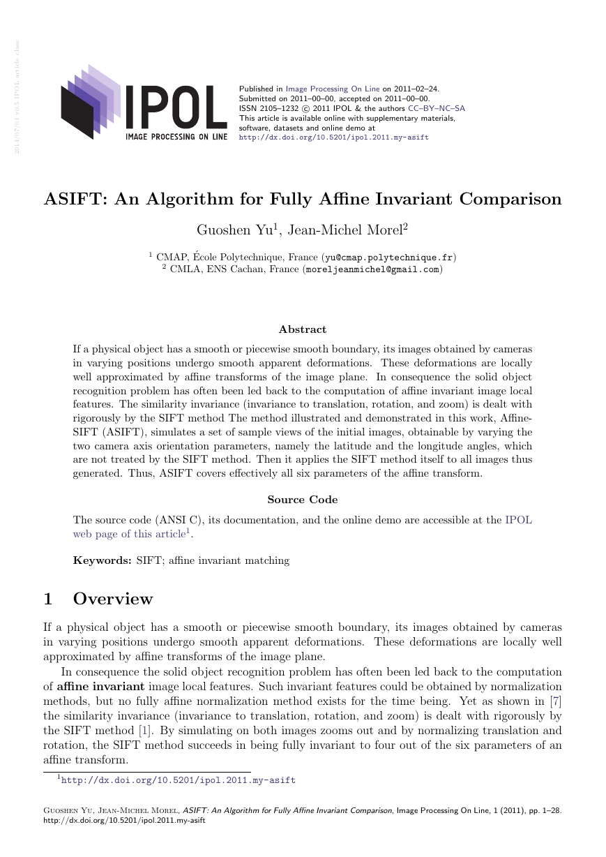
As illustrated by the camera model in Figure 1, digital image acquisition of a flat object can be
described as
u = S1G1AT u0,
where u is a digital image and u0 is an (ideal) infinite resolution frontal view of the flat object. The
parameters T and A are respectively a plane translation and a planar projective map due to the
camera motion. G1 is a Gaussian convolution modeling the optical blur, and S1 is the standard
sampling operator on a regular grid with mesh 1. The Gaussian kernel is assumed to be broad
enough to ensure no aliasing by the 1-sampling, therefore with a Shannon-Whittaker interpolation
I, one can recover the continuous image from its discrete version: IS1G1AT u0 = G1AT u0. S1 will
be thus omitted in the following.
3.2 Affine Local Approximation
We shall proceed to a further simplification of the above model, by reducing A to an affine map.
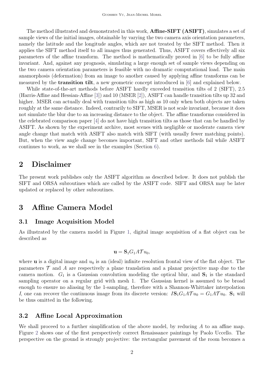
Figure 2 shows one of the first perspectively correct Renaissance paintings by Paolo Uccello. The
perspective on the ground is strongly projective: the rectangular pavement of the room becomes a
2
�
ASIFT: An Algorithm for Fully Affine Invariant Comparison
Figure 1: The projective camera model.
Figure 2: Affine local approximation.
trapezoid. However, each tile on the pavement is almost a parallelogram. This illustrates the local
tangency of perspective deformations to affine maps. Indeed, by the first order Taylor formula, any
planar smooth deformation can be approximated around each point by an affine map. The perspective
deformation of a plane object induced by a camera motion is a planar homographic transform, which
is smooth, and therefore locally tangent to affine transforms u(x, y) → u(ax + by + e, cx + dy + f ) in
each image region.
3.3 Affine Map Decomposition, with Geometric Interpretation as a Cam-
era Motion
Any affine map A with strictly positive determinant which is not a similarity has a unique decom-
position
A =
= HλR1(ψ)TtR2(φ) = λ
,
a b
c d
cos ψ − sin ψ
t 0
cos φ − sin φ
sin ψ cos ψ
0 1
sin φ cos φ
3
�
Guoshen Yu, Jean-Michel Morel
where λ > 0, λt is the determinant of A, Ri are rotations, φ ∈ [0, Π), and Tt is a tilt, namely a
diagonal matrix with first eigenvalue t > 1 and the second one equal to 1.
Figure 3: Geometric interpretation of affine decomposition.
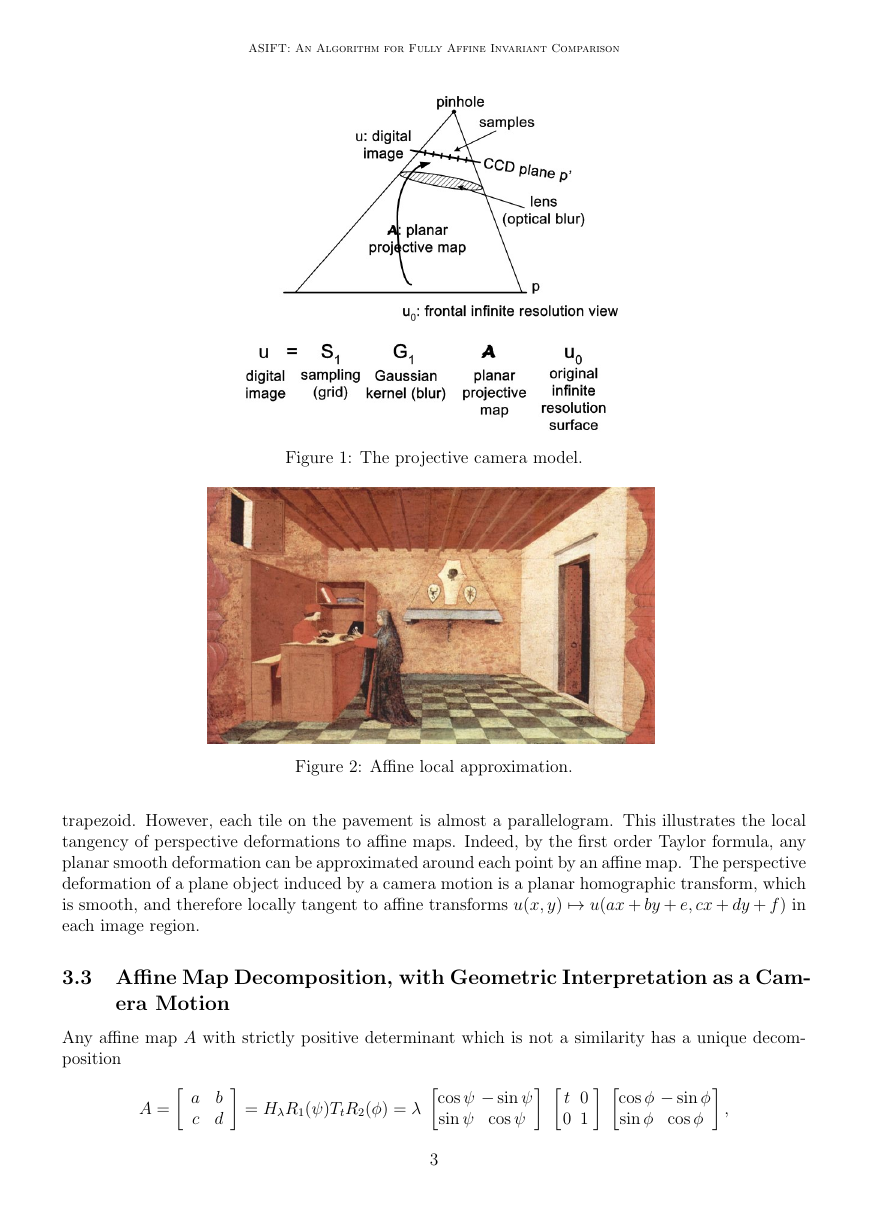
Figure 3 shows a camera motion interpretation of the affine decomposition: φ and θ = arccos 1/t
are the viewpoint angles, ψ parameterizes the camera spin and λ corresponds to the zoom. The
camera (the small parallelogram on the top-right) is assumed to stay far away from the image u
and starts from a frontal view u, i.e., λ = 1, t = 1, φ = ψ = 0. The camera can first move
parallel to the object’s plane: this motion induces a translation T that is eliminated by assuming
without loss of generality that the camera axis meets the image plane at a fixed point. The plane
containing the normal and the optical axis makes an angle φ with a fixed vertical plane. This angle
is called “longitude”. Its optical axis then makes a θ angle with the normal to the image plane u.
This parameter is called “latitude”. Both parameters are classical coordinates on the “observation
hemisphere”. The camera can rotate around its optical axis (rotation parameter ψ). Last but not
least, the camera can move forward or backward, as measured by the zoom parameter λ. We have
seen that the affine model is enough to give an account of local projective deformations. If the camera
were not assumed to be far away, the plane image deformation under a camera motion would be a
homography. Yet, as explained above, a homography is locally tangent to an affine map.
3.4 Transition Tilts, why can they be so High?
The parameter t defined above is called absolute tilt, since it measures the tilt between the frontal
view and a slanted view. In real applications, both compared images are usually slanted views. The
transition tilt is designed to quantify the amount of tilt between two such images. Assume that
v(x, y) = u(A(x, y)) and w(x, y) = u(B(x, y)) are two slanted views of a flat scene whose image is
u(x, y), where A and B are two affine maps. Then v(x, y) = w(AB−1(x, y)). The transition tilt
between v and w is defined as the absolute tilt associated with the affine map AB−1. Let t and t the
absolute tilts of two images u and u, and let φ and φ be their longitude angles. The transition tilt
τ (u, u) between the two images depends on the absolute tilts and the longitude angles, and satisfies
t/t ≤ τ (u, u) = τ (u, u) ≤ t t,
where we assume t ≥ t. The transition tilt can therefore be much higher than an absolute tilt.
Hence, it is important for an image matching algorithm to be invariant to high transition tilts.
4
�
ASIFT: An Algorithm for Fully Affine Invariant Comparison
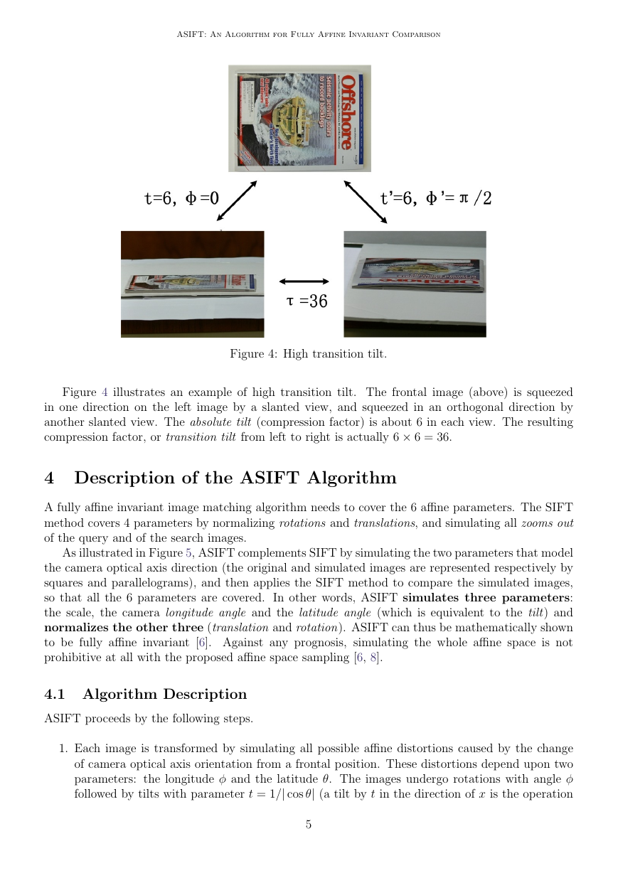
Figure 4: High transition tilt.
Figure 4 illustrates an example of high transition tilt. The frontal image (above) is squeezed
in one direction on the left image by a slanted view, and squeezed in an orthogonal direction by
another slanted view. The absolute tilt (compression factor) is about 6 in each view. The resulting
compression factor, or transition tilt from left to right is actually 6 × 6 = 36.
4 Description of the ASIFT Algorithm
A fully affine invariant image matching algorithm needs to cover the 6 affine parameters. The SIFT
method covers 4 parameters by normalizing rotations and translations, and simulating all zooms out
of the query and of the search images.
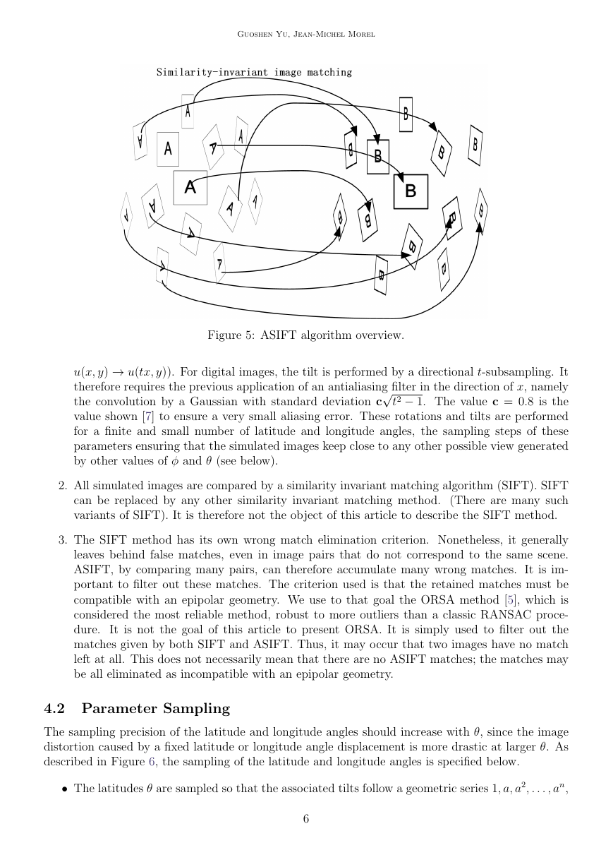
As illustrated in Figure 5, ASIFT complements SIFT by simulating the two parameters that model
the camera optical axis direction (the original and simulated images are represented respectively by
squares and parallelograms), and then applies the SIFT method to compare the simulated images,
so that all the 6 parameters are covered. In other words, ASIFT simulates three parameters:
the scale, the camera longitude angle and the latitude angle (which is equivalent to the tilt) and
normalizes the other three (translation and rotation). ASIFT can thus be mathematically shown
to be fully affine invariant [6]. Against any prognosis, simulating the whole affine space is not
prohibitive at all with the proposed affine space sampling [6, 8].
4.1 Algorithm Description
ASIFT proceeds by the following steps.
1. Each image is transformed by simulating all possible affine distortions caused by the change
of camera optical axis orientation from a frontal position. These distortions depend upon two
parameters: the longitude φ and the latitude θ. The images undergo rotations with angle φ
followed by tilts with parameter t = 1/| cos θ| (a tilt by t in the direction of x is the operation
5
�
Guoshen Yu, Jean-Michel Morel
Figure 5: ASIFT algorithm overview.
u(x, y) → u(tx, y)). For digital images, the tilt is performed by a directional t-subsampling. It
√
therefore requires the previous application of an antialiasing filter in the direction of x, namely
t2 − 1. The value c = 0.8 is the
the convolution by a Gaussian with standard deviation c
value shown [7] to ensure a very small aliasing error. These rotations and tilts are performed
for a finite and small number of latitude and longitude angles, the sampling steps of these
parameters ensuring that the simulated images keep close to any other possible view generated
by other values of φ and θ (see below).
2. All simulated images are compared by a similarity invariant matching algorithm (SIFT). SIFT
can be replaced by any other similarity invariant matching method. (There are many such
variants of SIFT). It is therefore not the object of this article to describe the SIFT method.
3. The SIFT method has its own wrong match elimination criterion. Nonetheless, it generally
leaves behind false matches, even in image pairs that do not correspond to the same scene.
ASIFT, by comparing many pairs, can therefore accumulate many wrong matches. It is im-
portant to filter out these matches. The criterion used is that the retained matches must be
compatible with an epipolar geometry. We use to that goal the ORSA method [5], which is
considered the most reliable method, robust to more outliers than a classic RANSAC proce-
dure.
It is not the goal of this article to present ORSA. It is simply used to filter out the
matches given by both SIFT and ASIFT. Thus, it may occur that two images have no match
left at all. This does not necessarily mean that there are no ASIFT matches; the matches may
be all eliminated as incompatible with an epipolar geometry.
4.2 Parameter Sampling
The sampling precision of the latitude and longitude angles should increase with θ, since the image
distortion caused by a fixed latitude or longitude angle displacement is more drastic at larger θ. As
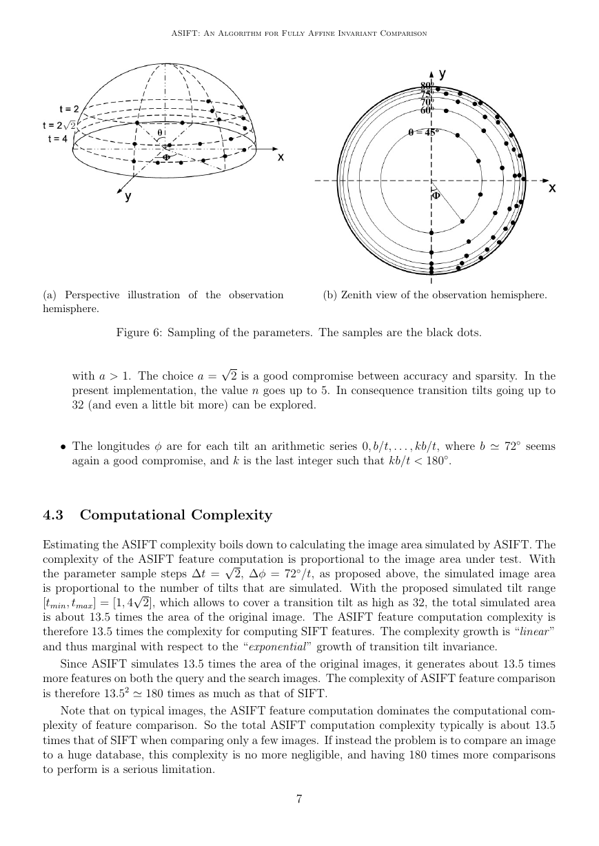
described in Figure 6, the sampling of the latitude and longitude angles is specified below.
• The latitudes θ are sampled so that the associated tilts follow a geometric series 1, a, a2, . . . , an,
6
�
ASIFT: An Algorithm for Fully Affine Invariant Comparison
(a) Perspective illustration of the observation
hemisphere.
(b) Zenith view of the observation hemisphere.
Figure 6: Sampling of the parameters. The samples are the black dots.
√
2 is a good compromise between accuracy and sparsity. In the
with a > 1. The choice a =
present implementation, the value n goes up to 5. In consequence transition tilts going up to
32 (and even a little bit more) can be explored.
• The longitudes φ are for each tilt an arithmetic series 0, b/t, . . . , kb/t, where b 72◦ seems
again a good compromise, and k is the last integer such that kb/t < 180◦.
4.3 Computational Complexity
√
Estimating the ASIFT complexity boils down to calculating the image area simulated by ASIFT. The
complexity of the ASIFT feature computation is proportional to the image area under test. With
2, ∆φ = 72◦/t, as proposed above, the simulated image area
the parameter sample steps ∆t =
√
is proportional to the number of tilts that are simulated. With the proposed simulated tilt range
2], which allows to cover a transition tilt as high as 32, the total simulated area
[tmin, tmax] = [1, 4
is about 13.5 times the area of the original image. The ASIFT feature computation complexity is
therefore 13.5 times the complexity for computing SIFT features. The complexity growth is “linear ”
and thus marginal with respect to the “exponential ” growth of transition tilt invariance.
Since ASIFT simulates 13.5 times the area of the original images, it generates about 13.5 times
more features on both the query and the search images. The complexity of ASIFT feature comparison
is therefore 13.52 180 times as much as that of SIFT.
Note that on typical images, the ASIFT feature computation dominates the computational com-
plexity of feature comparison. So the total ASIFT computation complexity typically is about 13.5
times that of SIFT when comparing only a few images. If instead the problem is to compare an image
to a huge database, this complexity is no more negligible, and having 180 times more comparisons
to perform is a serious limitation.
7
�
Guoshen Yu, Jean-Michel Morel
4.3.1 Coarse-to-fine Acceleration
An easy coarse-to-fine acceleration described in [6] reduces respectively the complexity of ASIFT
feature computation and comparison to 1.5 and 2.25 times that of SIFT. This acceleration is not
used here.
4.3.2 Parallelization
In addition, the SIFT subroutines (feature computation and comparison) in ASIFT are independent
and can easily be implemented in parallel. The online demo uses this possibility.
5
Implementation
5.1 ASIFT Feature Computation
Algorithm 1. Implemented in the C++ source file compute asift keypoints.cpp.
√
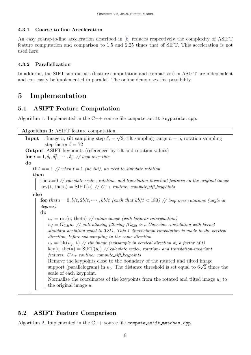
Algorithm 1: ASIFT feature computation.
2, tilt sampling range n = 5, rotation sampling
Input : Image u, tilt sampling step δt =
step factor b = 72
Output: ASIFT keypoints (referenced by tilt and rotation values)
for t = 1, δt, δ2
do
t // loop over tilts
t ,··· , δn
if t == 1 // when t = 1 (no tilt), no need to simulate rotation
then
theta=0 // calculate scale-, rotation- and translation-invariant features on the original image
key(t, theta) = SIFT(u) // C++ routine: compute sift keypoints
else
for theta = 0, b/t, 2b/t,··· , kb/t (such that kb/t < 180) // loop over rotations (angle in
degrees)
do
ur = rot(u, theta) // rotate image (with bilinear interpolation)
uf = G0.8tur // anti-aliasing filtering (G0.8t is a Gaussian convolution with kernel
standard deviation equal to 0.8t). This 1-dimensional convolution is made in the vertical
direction, before sub-sampling in the same direction.
ut = tilt(uf , t) // tilt image (subsample in vertical direction by a factor of t)
key(t, theta) = SIFT(ut) // calculate scale-, rotation- and translation-invariant
features. C++ routine: compute sift keypoints
Remove the keypoints close to the boundary of the rotated and tilted image
support (parallelogram) in ut. The distance threshold is set equal to 6
scale of each keypoint.
Normalize the coordinates of the keypoints from the rotated and tilted image ut to
the original image u.
√
2 times the
5.2 ASIFT Feature Comparison
Algorithm 2. Implemented in the C++ source file compute asift matches.cpp.
8
�


 2023年江西萍乡中考道德与法治真题及答案.doc
 2012年重庆南川中考生物真题及答案.doc
 2013年江西师范大学地理学综合及文艺理论基础考研真题.doc
 2020年四川甘孜小升初语文真题及答案I卷.doc
 2020年注册岩土工程师专业基础考试真题及答案.doc
 2023-2024学年福建省厦门市九年级上学期数学月考试题及答案.doc
 2021-2022学年辽宁省沈阳市大东区九年级上学期语文期末试题及答案.doc
 2022-2023学年北京东城区初三第一学期物理期末试卷及答案.doc
 2018上半年江西教师资格初中地理学科知识与教学能力真题及答案.doc
 2012年河北国家公务员申论考试真题及答案-省级.doc
 2020-2021学年江苏省扬州市江都区邵樊片九年级上学期数学第一次质量检测试题及答案.doc
 2022下半年黑龙江教师资格证中学综合素质真题及答案.doc