Vision Research 42 (2002) 1593–1605
www.elsevier.com/locate/visres
A multi-layer sparse coding network learns contour coding
from natural images q
Patrik O. Hoyer *, Aapo Hyv€aarinen
Neural Networks Research Centre, Helsinki University of Technology, P.O. Box 9800, FIN-02015 HUT, Finland
Received 17 April 2001; received in revised form 27 November 2001
Abstract
An important approach in visual neuroscience considers how the function of the early visual system relates to the statistics of its
natural input. Previous studies have shown how many basic properties of the primary visual cortex, such as the receptive fields of
simple and complex cells and the spatial organization (topography) of the cells, can be understood as efficient coding of natural
images. Here we extend the framework by considering how the responses of complex cells could be sparsely represented by a higher-
order neural layer. This leads to contour coding and end-stopped receptive fields. In addition, contour integration could be in-
terpreted as top-down inference in the presented model. Ó 2002 Elsevier Science Ltd. All rights reserved.
Keywords: Natural images; Neural networks; Contours; Cortex; Independent component analysis
1. Introduction
1.1. Why build statistical models of natural images?
After Hubel and Wiesel (1962, 1968) first showed that
neurons in mammalian primary visual cortex (V1) are
optimally stimulated by bars and edges, a large part of
visual neuroscience has been concerned with exploring
the response characteristics of neurons in V1 and in
higher visual areas. However, such studies do not di-
rectly answer the question of why the neurons respond
in the way that they do. Why does it make sense to filter
the incoming visual signals with receptive fields such as
those of V1 simple cells? What is the goal of the neural
code? Not only are such questions interesting in their
own right, but finding answers would give us a deeper
understanding of the information processing in the vi-
sual system and could even give predictions for neuronal
receptive fields in higher visual areas.
One important approach for answering such ques-
tions is to consider how the function of the visual system
relates to the properties of natural images. It has long
q This paper previously had the title: ‘A non-negative sparse coding
network learns contour coding and integration from natural images’.
The title was changed during revision.
* Corresponding author.
E-mail address: patrik.hoyer@hut.fi (P.O. Hoyer).
been hypothesized that the early visual system is adap-
ted to the input statistics (Attneave, 1954; Barlow,
1961). Such an adaptation is thought to be the result of
the combined forces of evolution and neural learning
during development. This hypothesis has lately been
gaining ground as information-theoretically efficient
coding strategies have been used to explain much of
the early processing of visual sensory data, including
response properties of neurons in the retina (Atick &
Redlich, 1992; Srinivasan, Laughlin, & Dubs, 1982),
lateral geniculate nucleus (Dan, Atick, & Reid, 1996;
Dong & Atick, 1995), and V1 (Bell & Sejnowski, 1997;
Hoyer & Hyv€aarinen, 2000; Hyv€aarinen & Hoyer, 2000,
2001; Olshausen & Field, 1996; Rao & Ballard, 1999;
Simoncelli & Schwartz, 1999; Tailor, Finkel, & Buchs-
baum, 2000; van Hateren & Ruderman, 1998; van
Hateren & van der Schaaf, 1998; Wachtler, Lee, & Sej-
nowski, 2001; Zetzsche & Krieger, 1999). For a recent
review, see (Simoncelli & Olshausen, 2001).
Although there seems to be a consensus that infor-
mation-theoretic arguments are relevant when investi-
gating the earliest parts of the visual system, there is no
general agreement on how far such arguments can be
taken. Can information theory be used to understand
neuronal processing higher in the processing ‘hierarchy’,
in, say, areas V2, V4, or perhaps even the inferotem-
poral cortex? One might, for instance, be inclined to
think that higher processes in the visual system would be
0042-6989/02/$ - see front matter Ó 2002 Elsevier Science Ltd. All rights reserved.
PII: S 0 0 4 2 - 6 9 8 9 ( 0 2 ) 0 0 0 1 7 - 2
�
1594
P.O. Hoyer, A. Hyv€aarinen / Vision Research 42 (2002) 1593–1605
X
n
i¼1
expected to be concerned with specific tasks (such as the
estimation of shape or heading) and not simply ‘repre-
senting the information efficiently’. Early levels, the ar-
gument goes, cannot be very goal oriented (as there are a
number of tasks that need to use that information) and
thus must simply concentrate on representing the in-
formation faithfully and efficiently.
We would like to suggest that emphasis should be
placed not on the hypothesis that the cortex simply seeks
to represent the sensory data efficiently, but rather on
the notion that it builds a probabilistic internal model
for those data. Such a change in emphasis from the
original redundancy reduction hypothesis has recently
been compellingly argued for by Barlow (2001a,b). 1
In such a framework, it is natural to think of neural
networks not as simply transforming the input signals
into coded representations having some desired prop-
erties (such as sparseness), but rather as modeling the
structure of the sensory data. Viewed in this light, data-
driven probabilistic models make as much sense at
higher levels of the processing hierarchy as at the earliest
stages of the visual system. Although not being the focus
of the large majority of work on sensory coding (re-
viewed in Simoncelli & Olshausen, 2001), this point of
view has nonetheless been emphasized by a number of
researchers (see e.g. Dayan, Hinton, Neal, & Zemel,
1995; Hinton, Dayan, Frey, & Neal, 1995; Hinton &
Ghahramani, 1997; Mumford, 1994; Olshausen & Field,
1997; Rao & Ballard, 1999) and is also the approach we
take.
1.2. Modeling V1 receptive fields with sparse coding
In an influential paper, Olshausen and Field (1996)
showed how the classical receptive fields of simple cells
in V1 can be understood in the framework of sparse
coding. The basic idea is to model the observed data
(random variables) xj as a weighted sum of some hidden
(latent) random variables si, to which Gaussian noise
has been added: 2
xj ¼
ajisi þ nj:
ð1Þ
X
n
i¼1
x ¼
aisi þ n:
ð2Þ
In other words, each observed data pattern x is ap-
proximately expressed as some linear combination of the
basis patterns ai. The hidden variables si that give the
mixing proportions are stochastic and differ for each
observed x.
The crucial assumption in the sparse coding frame-
work is that the hidden random variables si are mutually
independent and that they exhibit sparseness. Sparseness
is a property independent of scale (variance), and im-
plies that the si have probability densities which are
highly peaked at zero and have heavy tails. Essentially,
the idea is that any single typical input pattern x can be
accurately described using only a few active (signifi-
cantly non-zero) units si. However, all of the basis pat-
terns ai are needed to represent the data because the set
of active units changes from input to input.
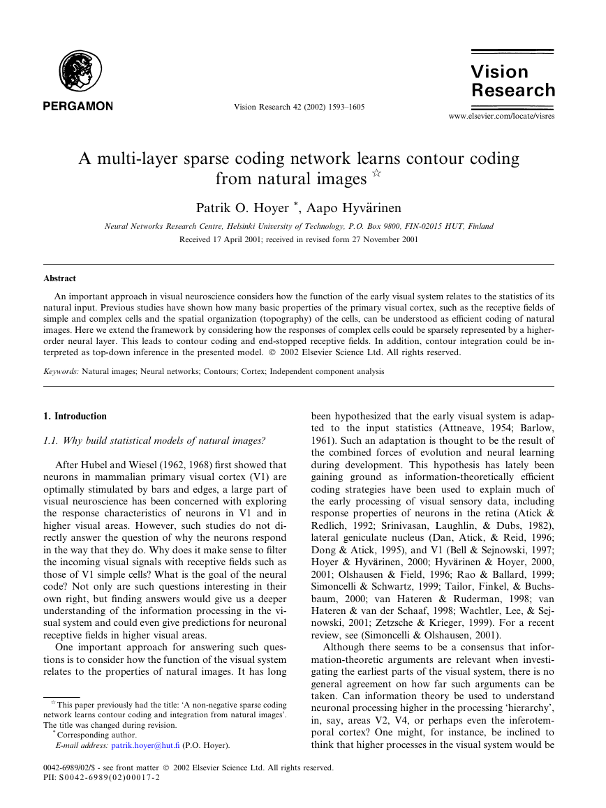
This model can be represented by a simple neural
network (see Fig. 1), where the observed data x (repre-
sented by the activities in the lower, input layer) are a
linear function of the activities of the hidden variables si
in the higher layer, contaminated by additive Gaussian
noise (Olshausen & Field, 1997). Upon observing an
input x, the network calculates the optimal representa-
tion si in the sense that it is the configuration of the
hidden variables most likely to have caused the observed
data. This is inferring the latent variables, and is the
short-timescale goal of the network. Since the prior
probability of the si is sparse, this boils down to finding
a maximally sparse configuration of the si that never-
theless approximately generates x. In the long run, the
goal of the network is to learn (adapt) the generative
weights (basis patterns) ai so that the probability of the
data is maximized. Again, for sparse latent variables,
this is achieved when the weights are such that only a
few higher-layer neurons si need to be significantly ac-
tive to represent typical input patterns.
When the network is trained on data consisting of
patches from natural images, with the elements of x
representing pixel grayscale values, the learned basis
This can be expressed compactly in vector form (with
bold letters indicating vector quantities) as
1 Of course, information theory tells us that the better model we
have for some given data, the more efficiently (compactly) we could
potentially represent it. However, for the case of the brain, it may well
be that it is the model that is important, not the forming of a compact
representation.
2 This sparse coding model is also called the noisy independent
component analysis (ICA) model (Hyv€aarinen, Karhunen, & Oja,
2001).
Fig. 1. The linear sparse coding neural network. Units are depicted by
filled circles, and arrows represent conditional dependencies (in the
generative model) between the units. Upon observing data x the hid-
den neuron activities si are calculated as the most probable latent
variable values to have generated the data. On a longer timescale, the
generative weights aij are adapted to allow typical data to be repre-
sented sparsely.
�
P.O. Hoyer, A. Hyv€aarinen / Vision Research 42 (2002) 1593–1605
1595
patterns ai resemble Gabor functions and V1 simple cell
classical receptive fields, and the corresponding si can be
interpreted as the activations of the cells (Bell & Sej-
nowski, 1997; Olshausen & Field, 1996; van Hateren &
van der Schaaf, 1998). This basic result has already
been extended to explain spatiotemporal (van Hateren &
Ruderman, 1998), chromatic (Hoyer & Hyv€aarinen, 2000;
Tailor et al., 2000; Wachtler et al., 2001), and binocular
(Hoyer & Hyv€aarinen, 2000) properties of simple cells.
This can be done simply by training the network on
input data consisting of image sequences, colour images,
and stereo images, respectively.
Although the basic sparse coding model has been
quite successful at explaining the receptive fields of
simple cells in V1, it is not difficult to see that it cannot
account for the behaviour of V1 complex cells. These
cells are, just as simple cells, sensitive to the orientation
and spatial frequency of the stimulus, but unlike simple
cells they are not very sensitive to the phase of the
stimulus. Such invariance is impossible to describe with a
strictly linear model. Consider, for instance, reversing
of contrast polarity of the stimulus. Such an operation
would flip the sign of a linear representation, whereas
the response of a typical complex cell does not change
to any significant degree.
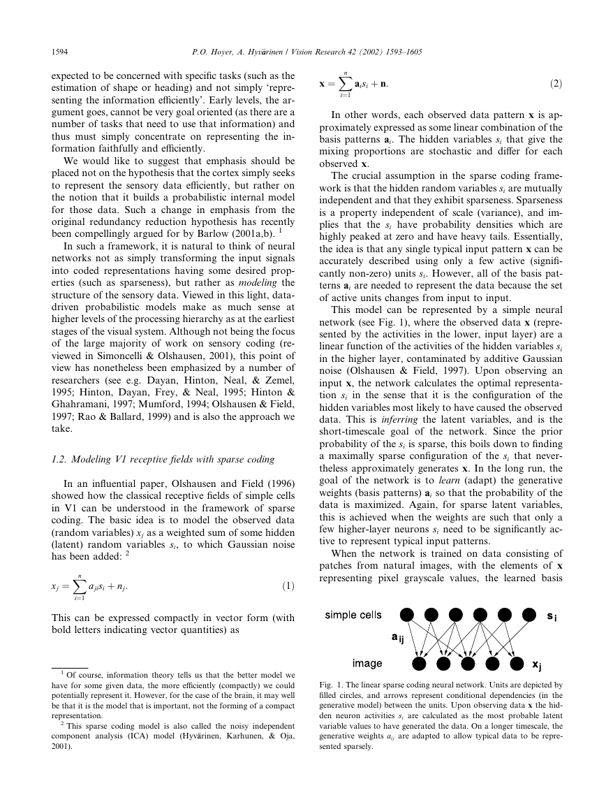
To model such stimulus invariance, Hyv€aarinen and
Hoyer (2000) modified the network to include higher-
order cells that pooled the energies (squared outputs) of
groups of simple cells. Such pooling can be interpreted
as a generative model in which the higher-order cells
determine the variances of the simple cells (Hyv€aarinen,
Hoyer, & Inki, 2001). This model is depicted in Fig. 2.
(Note that simply adding a second linear layer on top of
the first one would not be very useful, because a linear
transform followed by another linear transform is still a
linear transform, so nothing is gained by a multi-layer
network.) When trained on natural image patches, the
adaptable weights ai converged to simple cell-like re-
ceptive fields, and the behaviour of the higher-order
units was qualitatively similar to complex cell re-
sponses. 3 This behaviour was due to the fact that simple
cells in any single group learned receptive fields of
similar orientation and spatial frequency, but differing
spatial phase. A further extension was introduced in
(Hyv€aarinen & Hoyer, 2001; Hyv€aarinen et al., 2001),
where it was shown how V1-like topography can addi-
tionally emerge.
1.3. A multi-layer model
An important question is how to extend these models
to account for response properties of neurons higher in
3 The model actually estimated in (Hyv€aarinen & Hoyer, 2000) was a
simplified version where there was no noise and the number of hidden
variables si was equal to the dimensionality of the data.
Fig. 2. The extended sparse coding model (Hyv€aarinen & Hoyer, 2000;
Hyv€aarinen et al., 2001). Each complex cell determines the variance of a
group of simple cells.
the processing hierarchy. Perhaps the most straightfor-
ward approach is to add a linear layer on top of the
complex cell model. This would amount to assuming a
model where the activities of our model complex cells
are not independent, but rather can be described as a
linear combination of some higher-order independent
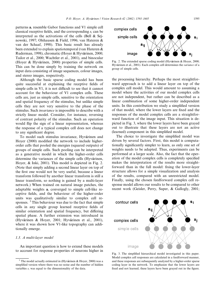
units. In this contribution we study a simplified version
of that model, where the lower layers are fixed and the
responses of the model complex cells are a straightfor-
ward function of the image input. This situation is de-
picted in Fig. 3, where the lower layers have been grayed
out to illustrate that these layers are not an active
(learned) component in this simplified model.
The choice to investigate the simplified model was
driven by several factors. First, this model is computa-
tionally significantly simpler to learn, as only one set of
weights needs to be adapted. Thus, experiments can be
performed at a larger scale. Also, the fact that the oper-
ation of the model complex cells is completely specified
makes the interpretation of the results more straight-
forward than in the full model: fixing the lower-layer
structure allows for a simple visualization and analysis
of the results, compared with an unrestricted model.
Finally, using the chosen feedforward complex cell re-
sponse model allows our results to be compared to other
recent work (Geisler, Perry, Super, & Gallogly, 2001;
Fig. 3. The simplified hierarchical model investigated in this paper.
Model complex cell responses are calculated in a feedforward manner,
and these responses are subsequently analyzed by a higher-order sparse
coding layer in the network. To emphasize that the lower layers are
fixed and not learned, these layers have been grayed out in the figure.
�
1596
P.O. Hoyer, A. Hyv€aarinen / Vision Research 42 (2002) 1593–1605
Kr€uuger, 1998; Sigman, Cecchi, Gilbert, & Magnasco,
2001) analyzing the dependencies of complex cell re-
sponses. We believe that the analysis provided in this
paper can be viewed as a preliminary investigation into
how complex cell responses could be represented in an
unrestricted multi-layer model.
In brief, we model V1 complex cell outputs by a
classic complex cell energy model and, using these re-
sponses as the input x, estimate the linear model of Eq.
(2) assuming sparse, non-negative si. We show how our
network learns contour coding from natural images in
an unsupervised fashion, and discuss how contour in-
tegration could be viewed as resulting from top-down
inference in the model.
2. Methods
2.1. Model complex cells
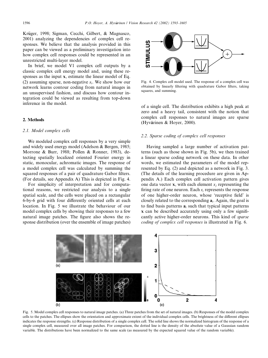
We modeled complex cell responses by a very simple
and widely used energy model (Adelson & Bergen, 1985;
Morrone & Burr, 1988; Pollen & Ronner, 1983), de-
tecting spatially localized oriented Fourier energy in
static, monocular, achromatic images. The response of
a model complex cell was calculated by summing the
squared responses of a pair of quadrature Gabor filters.
(For details, see Appendix A) This is depicted in Fig. 4.
For simplicity of interpretation and for computa-
tional reasons, we restricted our analysis to a single
spatial scale, and the cells were placed on a rectangular
6-by-6 grid with four differently oriented cells at each
location. In Fig. 5 we illustrate the behaviour of our
model complex cells by showing their responses to a few
natural image patches. The figure also shows the re-
sponse distribution (over the ensemble of image patches)
Fig. 4. Complex cell model used. The response of a complex cell was
obtained by linearly filtering with quadrature Gabor filters, taking
squares, and summing.
of a single cell. The distribution exhibits a high peak at
zero and a heavy tail, consistent with the notion that
complex cell responses to natural
images are sparse
(Hyv€aarinen & Hoyer, 2000).
2.2. Sparse coding of complex cell responses
Having sampled a large number of activation pat-
terns (such as those shown in Fig. 5b), we then trained
a linear sparse coding network on these data. In other
words, we estimated the parameters of the model rep-
resented by Eq. (2) and depicted as a network in Fig. 3.
(The details of the learning procedure are given in Ap-
pendix A.) Each complex cell activation pattern gives
one data vector x, with each element xj representing the
firing rate of one neuron. Each si represents the response
of one higher-order neuron, whose ‘receptive field’ is
closely related to the corresponding ai. Again, the goal is
to find basis patterns ai such that typical input patterns
x can be described accurately using only a few signifi-
cantly active higher-order neurons. This kind of sparse
coding of complex cell responses is illustrated in Fig. 6.
Fig. 5. Model complex cell responses to natural image patches. (a) Three patches from the set of natural images. (b) Responses of the model complex
cells to the patches. The ellipses show the orientation and approximate extent of the individual complex cells. The brightness of the different ellipses
indicates the response strengths. (c) Response distribution of a single complex cell. The solid line shows the normalized histogram of the response of a
single complex cell, measured over all image patches. For comparison, the dotted line is the density of the absolute value of a Gaussian random
variable. The distributions have been normalized to the same scale (as measured by the expected squared value of the random variable).
�
P.O. Hoyer, A. Hyv€aarinen / Vision Research 42 (2002) 1593–1605
1597
Fig. 6. Sparse coding of complex cell responses. Each complex cell activity pattern is represented as a linear combination of basis patterns ai. The
goal is to find basis patterns such that the coefficients si are as ‘sparse’ as possible, meaning that for most input patterns only a few of them are needed
to represent the pattern accurately. Cf. Eq. (2).
Because our input data (complex cell responses)
cannot go negative it is natural to require our generative
representation to be non-negative. Thus both the ai and
the si were restricted to non-negative values. 4 Argu-
ments for non-negative representations (Paatero &
Tapper, 1994) have previously been presented by Lee
and Seung (1999). However, in contrast to their ap-
proach, we emphasize the importance of sparseness
in addition to good reconstruction. Such emphasis on
sparseness has previously been forcefully argued for by
Barlow (1972) and Field (1994). Thus, we combine
sparse coding and the constraint of non-negativity into a
single model. Note that neither assumption is arbitrary;
both follow from the properties of complex cell re-
sponses, which are sparse and non-negative.
3. Results
3.1. Properties of the learned representation
Using simulated complex cell responses to natural
images as input data (see Fig. 5), we thus estimated the
non-negative sparse coding model, obtaining 288 basis
(activity) patterns. A representative subset of the esti-
mated basis patterns ai is shown in Fig. 7. Note that
most basis patterns consist of a variable number of ac-
tive complex cells arranged collinearly. This makes in-
tuitive sense, as collinearity is a strong feature of the
visual world (Geisler et al., 2001; Kr€uuger, 1998; Sigman
et al., 2001). In addition, analyzing images in terms of
smooth contours is supported by evidence from both
psychophysics (Field, Hayes, & Hess, 1993; Polat &
Sagi, 1993) and physiology (Kapadia, Ito, Gilbert, &
Westheimer, 1995; Kapadia, Westheimer, & Gilbert,
2000; Polat, Mizobe, Pettet, Kasamatsu, & Norcia,
1998), and is incorporated in many models of contour
integration, see e.g. (Grossberg & Mingolla, 1985; Li,
1999; Neumann & Sepp, 1999). To our knowledge, ours
4 Allowing either ai or si to take negative values would imply that
our model would assign non-zero probability density to negative x. As
our data are non-negative it therefore makes sense to require the same
of both the basis and the coefficients. In our experiments, however, we
noted that the non-negativity constraint on the ai was not strictly
necessary, as the ai tended to be positive even without the constraint.
Rather, it is the constraint on the si that is crucial.
Fig. 7. A representative set of basis functions from the learned basis.
The majority of units code the simultaneous activation of collinear
complex cells, indicating a smooth contour in the image.
is the first model to learn this type of a representation
from the statistics of natural images.
It is easy to understand why basis patterns consist of
collinear complex cell activity patterns: such patterns are
typical in the data set, and can be sparsely coded if a
long contour can be represented by only a few higher-
level units. The necessity for different length basis pat-
terns comes from the fact that long basis patterns simply
cannot code short (or curved) contours, and short basis
patterns are inefficient at representing long, straight
contours. This kind of contour coding is illustrated in
Fig. 8.
Fig. 8. Contour coding in the model. A hypothetical contour in an
image (left) is transformed into complex cell responses (middle). These
responses can be sparsely represented using only three higher-order
units (right) of the types shown in Fig. 7.
�
1598
P.O. Hoyer, A. Hyv€aarinen / Vision Research 42 (2002) 1593–1605
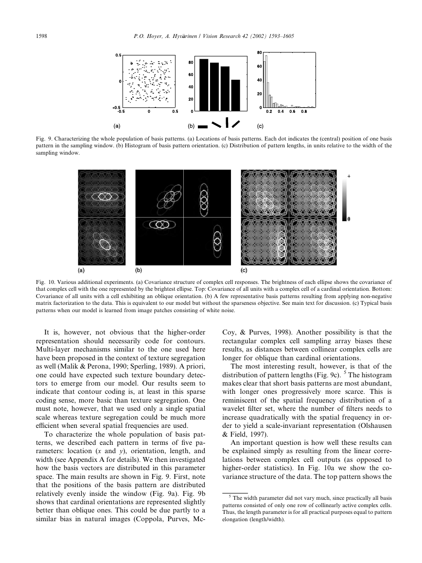
Fig. 9. Characterizing the whole population of basis patterns. (a) Locations of basis patterns. Each dot indicates the (central) position of one basis
pattern in the sampling window. (b) Histogram of basis pattern orientation. (c) Distribution of pattern lengths, in units relative to the width of the
sampling window.
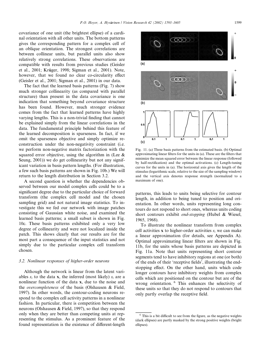
Fig. 10. Various additional experiments. (a) Covariance structure of complex cell responses. The brightness of each ellipse shows the covariance of
that complex cell with the one represented by the brightest ellipse. Top: Covariance of all units with a complex cell of a cardinal orientation. Bottom:
Covariance of all units with a cell exhibiting an oblique orientation. (b) A few representative basis patterns resulting from applying non-negative
matrix factorization to the data. This is equivalent to our model but without the sparseness objective. See main text for discussion. (c) Typical basis
patterns when our model is learned from image patches consisting of white noise.
It is, however, not obvious that the higher-order
representation should necessarily code for contours.
Multi-layer mechanisms similar to the one used here
have been proposed in the context of texture segregation
as well (Malik & Perona, 1990; Sperling, 1989). A priori,
one could have expected such texture boundary detec-
tors to emerge from our model. Our results seem to
indicate that contour coding is, at least in this sparse
coding sense, more basic than texture segregation. One
must note, however, that we used only a single spatial
scale whereas texture segregation could be much more
efficient when several spatial frequencies are used.
To characterize the whole population of basis pat-
terns, we described each pattern in terms of five pa-
rameters: location (x and y), orientation, length, and
width (see Appendix A for details). We then investigated
how the basis vectors are distributed in this parameter
space. The main results are shown in Fig. 9. First, note
that the positions of the basis pattern are distributed
relatively evenly inside the window (Fig. 9a). Fig. 9b
shows that cardinal orientations are represented slightly
better than oblique ones. This could be due partly to a
similar bias in natural images (Coppola, Purves, Mc-
Coy, & Purves, 1998). Another possibility is that the
rectangular complex cell sampling array biases these
results, as distances between collinear complex cells are
longer for oblique than cardinal orientations.
The most interesting result, however, is that of the
distribution of pattern lengths (Fig. 9c). 5 The histogram
makes clear that short basis patterns are most abundant,
with longer ones progressively more scarce. This is
reminiscent of the spatial frequency distribution of a
wavelet filter set, where the number of filters needs to
increase quadratically with the spatial frequency in or-
der to yield a scale-invariant representation (Olshausen
& Field, 1997).
An important question is how well these results can
be explained simply as resulting from the linear corre-
lations between complex cell outputs (as opposed to
higher-order statistics). In Fig. 10a we show the co-
variance structure of the data. The top pattern shows the
5 The width parameter did not vary much, since practically all basis
patterns consisted of only one row of collinearly active complex cells.
Thus, the length parameter is for all practical purposes equal to pattern
elongation (length/width).
�
P.O. Hoyer, A. Hyv€aarinen / Vision Research 42 (2002) 1593–1605
1599
covariance of one unit (the brightest ellipse) of a cardi-
nal orientation with all other units. The bottom patterns
gives the corresponding pattern for a complex cell of
an oblique orientation. The strongest correlations are
between collinear units, but parallel units also show
relatively strong correlations. These observations are
compatible with results from previous studies (Geisler
et al., 2001; Kr€uuger, 1998; Sigman et al., 2001). Note,
however, that we found no clear co-circularity effect
(Geisler et al., 2001; Sigman et al., 2001) in our data.
The fact that the learned basis patterns (Fig. 7) show
much stronger collinearity (as compared with parallel
structure) than present in the data covariance is one
indication that something beyond covariance structure
has been found. However, much stronger evidence
comes from the fact that learned patterns have highly
varying lengths. This is a non-trivial finding that cannot
be explained simply from the linear correlations in the
data. The fundamental principle behind this feature of
the learned decomposition is sparseness. In fact, if we
omit the sparseness objective and simply optimize re-
construction under the non-negativity constraint (i.e.
we perform non-negative matrix factorization with the
squared error objective, using the algorithm in (Lee &
Seung, 2001)) we do get collinearity but not any signif-
icant variation in basis pattern lengths. (For illustration,
a few such basis patterns are shown in Fig. 10b.) We will
return to the length distribution in Section 3.2.
A second question is whether the dependencies ob-
served between our model complex cells could be to a
significant degree due to the particular choice of forward
transform (the complex cell model and the chosen
sampling grid) and not natural image statistics. To in-
vestigate this we fed our network with image patches
consisting of Gaussian white noise, and examined the
learned basis patterns; a small subset is shown in Fig.
10c. These basis patterns exhibited only a very low
degree of collinearity and were not localized inside the
patch. This shows clearly that our results are for the
most part a consequence of the input statistics and not
simply due to the particular complex cell transform
chosen.
3.2. Nonlinear responses of higher-order neurons
Although the network is linear from the latent vari-
ables si to the data x, the inferred (most likely) si are a
nonlinear function of the data x, due to the noise and
the overcompleteness of the basis (Olshausen & Field,
1997). In other words, the contour-coding neurons re-
spond to the complex cell activity patterns in a nonlinear
fashion. In particular, there is competition between the
neurons (Olshausen & Field, 1997), so that they respond
only when they are better than competing units at rep-
resenting the stimulus. As a prominent feature of the
found representation is the existence of different-length
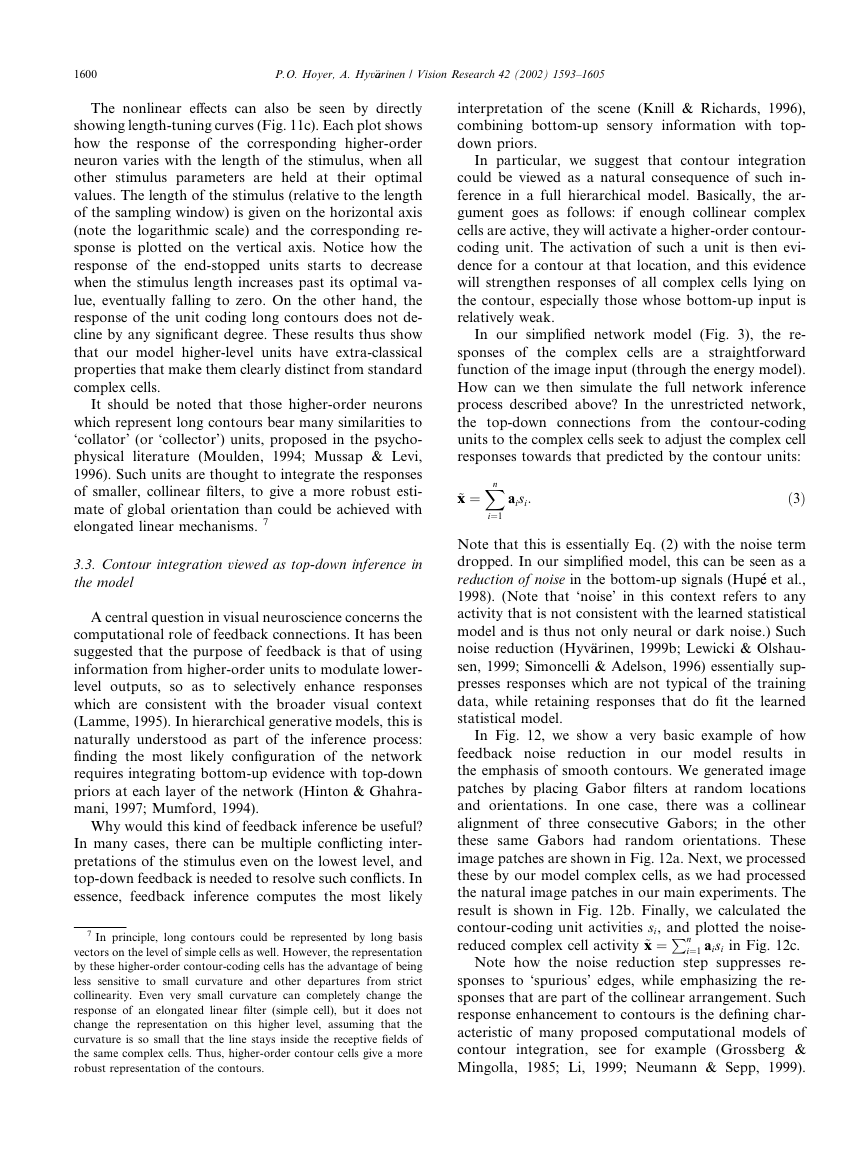
Fig. 11. (a) Three basis patterns from the estimated basis. (b) Optimal
approximating linear filters for the units in (a). These are the filters that
minimize the mean squared error between the linear response (followed
by half-rectification) and the optimal activations. (c) Length-tuning
curves for the units in (a). The horizontal axis gives the length of the
stimulus (logarithmic scale, relative to the size of the sampling window)
and the vertical axis denotes response strength (normalized to a
maximum of one).
patterns, this leads to units being selective for contour
length, in addition to being tuned to position and ori-
entation. In other words, units representing long con-
tours do not respond to short ones, whereas units coding
short contours exhibit end-stopping (Hubel & Wiesel,
1965, 1968).
To illustrate the nonlinear transform from complex
cell activities x to higher-order activities si we can make
a linear approximation (for details, see Appendix A).
Optimal approximating linear filters are shown in Fig.
11b, for the units whose basis patterns are depicted in
Fig. 11a. Note that units representing short contour
segments tend to have inhibitory regions at one (or both)
of the ends of their ‘receptive fields’, illustrating the end-
stopping effect. On the other hand, units which code
longer contours have inhibitory weights from complex
cells which are positioned on the contour but are of the
wrong orientation. 6 This enhances the selectivity of
these units so that they do not respond to contours that
only partly overlap the receptive field.
6 This is a bit difficult to see from the figure, as the negative weights
(dark ellipses) are partly masked by the strong positive weights (bright
ellipses).
�
1600
P.O. Hoyer, A. Hyv€aarinen / Vision Research 42 (2002) 1593–1605
The nonlinear effects can also be seen by directly
showing length-tuning curves (Fig. 11c). Each plot shows
how the response of the corresponding higher-order
neuron varies with the length of the stimulus, when all
other stimulus parameters are held at their optimal
values. The length of the stimulus (relative to the length
of the sampling window) is given on the horizontal axis
(note the logarithmic scale) and the corresponding re-
sponse is plotted on the vertical axis. Notice how the
response of the end-stopped units starts to decrease
when the stimulus length increases past its optimal va-
lue, eventually falling to zero. On the other hand, the
response of the unit coding long contours does not de-
cline by any significant degree. These results thus show
that our model higher-level units have extra-classical
properties that make them clearly distinct from standard
complex cells.
It should be noted that those higher-order neurons
which represent long contours bear many similarities to
‘collator’ (or ‘collector’) units, proposed in the psycho-
physical
literature (Moulden, 1994; Mussap & Levi,
1996). Such units are thought to integrate the responses
of smaller, collinear filters, to give a more robust esti-
mate of global orientation than could be achieved with
elongated linear mechanisms. 7
3.3. Contour integration viewed as top-down inference in
the model
A central question in visual neuroscience concerns the
computational role of feedback connections. It has been
suggested that the purpose of feedback is that of using
information from higher-order units to modulate lower-
level outputs, so as to selectively enhance responses
which are consistent with the broader visual context
(Lamme, 1995). In hierarchical generative models, this is
naturally understood as part of the inference process:
finding the most likely configuration of the network
requires integrating bottom-up evidence with top-down
priors at each layer of the network (Hinton & Ghahra-
mani, 1997; Mumford, 1994).
Why would this kind of feedback inference be useful?
In many cases, there can be multiple conflicting inter-
pretations of the stimulus even on the lowest level, and
top-down feedback is needed to resolve such conflicts. In
essence, feedback inference computes the most likely
7 In principle, long contours could be represented by long basis
vectors on the level of simple cells as well. However, the representation
by these higher-order contour-coding cells has the advantage of being
less sensitive to small curvature and other departures from strict
collinearity. Even very small curvature can completely change the
response of an elongated linear filter (simple cell), but it does not
change the representation on this higher level, assuming that the
curvature is so small that the line stays inside the receptive fields of
the same complex cells. Thus, higher-order contour cells give a more
robust representation of the contours.
interpretation of the scene (Knill & Richards, 1996),
combining bottom-up sensory information with top-
down priors.
In particular, we suggest that contour integration
could be viewed as a natural consequence of such in-
ference in a full hierarchical model. Basically, the ar-
gument goes as follows: if enough collinear complex
cells are active, they will activate a higher-order contour-
coding unit. The activation of such a unit is then evi-
dence for a contour at that location, and this evidence
will strengthen responses of all complex cells lying on
the contour, especially those whose bottom-up input is
relatively weak.
In our simplified network model (Fig. 3), the re-
sponses of the complex cells are a straightforward
function of the image input (through the energy model).
How can we then simulate the full network inference
process described above? In the unrestricted network,
the top-down connections from the contour-coding
units to the complex cells seek to adjust the complex cell
responses towards that predicted by the contour units:
ð3Þ
X
n
~xx ¼
aisi:
i¼1
Note that this is essentially Eq. (2) with the noise term
dropped. In our simplified model, this can be seen as a
reduction of noise in the bottom-up signals (Hup�ee et al.,
1998). (Note that ‘noise’ in this context refers to any
activity that is not consistent with the learned statistical
model and is thus not only neural or dark noise.) Such
noise reduction (Hyv€aarinen, 1999b; Lewicki & Olshau-
sen, 1999; Simoncelli & Adelson, 1996) essentially sup-
presses responses which are not typical of the training
data, while retaining responses that do fit the learned
statistical model.
In Fig. 12, we show a very basic example of how
feedback noise reduction in our model results in
the emphasis of smooth contours. We generated image
patches by placing Gabor filters at random locations
and orientations. In one case, there was a collinear
alignment of three consecutive Gabors;
in the other
these same Gabors had random orientations. These
image patches are shown in Fig. 12a. Next, we processed
these by our model complex cells, as we had processed
the natural image patches in our main experiments. The
result is shown in Fig. 12b. Finally, we calculated the
contour-coding unit activities si, and plotted the noise-
reduced complex cell activity ~xx ¼
n
i¼1 aisi in Fig. 12c.
Note how the noise reduction step suppresses re-
sponses to ‘spurious’ edges, while emphasizing the re-
sponses that are part of the collinear arrangement. Such
response enhancement to contours is the defining char-
acteristic of many proposed computational models of
contour integration, see for example (Grossberg &
Mingolla, 1985; Li, 1999; Neumann & Sepp, 1999).
P
�



 2023年江西萍乡中考道德与法治真题及答案.doc
 2012年重庆南川中考生物真题及答案.doc
 2013年江西师范大学地理学综合及文艺理论基础考研真题.doc
 2020年四川甘孜小升初语文真题及答案I卷.doc
 2020年注册岩土工程师专业基础考试真题及答案.doc
 2023-2024学年福建省厦门市九年级上学期数学月考试题及答案.doc
 2021-2022学年辽宁省沈阳市大东区九年级上学期语文期末试题及答案.doc
 2022-2023学年北京东城区初三第一学期物理期末试卷及答案.doc
 2018上半年江西教师资格初中地理学科知识与教学能力真题及答案.doc
 2012年河北国家公务员申论考试真题及答案-省级.doc
 2020-2021学年江苏省扬州市江都区邵樊片九年级上学期数学第一次质量检测试题及答案.doc
 2022下半年黑龙江教师资格证中学综合素质真题及答案.doc