0
2
0
2
r
a
M
1
1
]
V
C
.
s
c
[
3
v
9
6
1
0
0
.
9
0
9
1
:
v
i
X
r
a
OKSUZ et al.: IMBALANCE PROBLEMS IN OBJECT DETECTION: A REVIEW
1
Imbalance Problems in Object Detection: A
Review
Kemal Oksuz†
, Baris Can Cam , Sinan Kalkan‡
, and Emre Akbas‡
Abstract—In this paper, we present a comprehensive review of the imbalance problems in object detection. To analyze the problems in
a systematic manner, we introduce a problem-based taxonomy. Following this taxonomy, we discuss each problem in depth and
present a unifying yet critical perspective on the solutions in the literature. In addition, we identify major open issues regarding the
existing imbalance problems as well as imbalance problems that have not been discussed before. Moreover, in order to keep our
review up to date, we provide an accompanying webpage which catalogs papers addressing imbalance problems, according to our
problem-based taxonomy. Researchers can track newer studies on this webpage available at:
https://github.com/kemaloksuz/ObjectDetectionImbalance.
!
1 INTRODUCTION
Object detection is the simultaneous estimation of categories
and locations of object instances in a given image. It is a fun-
damental problem in computer vision with many important
applications in e.g. surveillance [1], [2], autonomous driving
[3], [4], medical decision making [5], [6], and many problems
in robotics [7], [8], [9], [10], [11], [12].
Since the time when object detection (OD) was cast as
a machine learning problem, the first generation OD meth-
ods relied on hand-crafted features and linear, max-margin
classifiers. The most successful and representative method
in this generation was the Deformable Parts Model (DPM)
[13]. After the extremely influential work by Krizhevsky et
al. in 2012 [14], deep learning (or deep neural networks) has
started to dominate various problems in computer vision
and OD was no exception. The current generation OD
methods are all based on deep learning where both the
hand-crafted features and linear classifiers of the first gener-
ation methods have been replaced by deep neural networks.
This replacement has brought significant improvements in
performance: On a widely used OD benchmark dataset
(PASCAL VOC), while the DPM [13] achieved 0.34 mean
average-precision (mAP), current deep learning based OD
models achieve around 0.80 mAP [15].
In the last five years, although the major driving force of
progress in OD has been the incorporation of deep neural
networks [16], [17], [18], [19], [20], [21], [22], [23], imbalance
problems in OD at several levels have also received signif-
icant attention [24], [25], [26], [27], [28], [29], [30]. An im-
balance problem with respect to an input property occurs
when the distribution regarding that property affects the
performance. When not addressed, an imbalance problem
has adverse effects on the final detection performance. For
example, the most commonly known imbalance problem
in OD is the foreground-to-background imbalance which
All authors are at the Dept. of Computer Engineering, Middle East Techni-
cal University (METU), Ankara, Turkey. E-mail:{kemal.oksuz@metu.edu.tr,
can.cam@metu.edu.tr, skalkan@metu.edu.tr, emre@ceng.metu.edu.tr}
† Corresponding author.
‡ Equal contribution for senior authorship.
manifests itself in the extreme inequality between the num-
ber of positive examples versus the number of negatives.
In a given image, while there are typically a few positive
examples, one can extract millions of negative examples.
If not addressed, this imbalance greatly impairs detection
accuracy.
In this paper, we review the deep-learning-era object
detection literature and identify eight different imbalance
problems. We group these problems in a taxonomy with
four main types: class imbalance, scale imbalance, spatial
imbalance and objective imbalance (Table 1). Class imbal-
ance occurs when there is significant inequality among
the number of examples pertaining to different classes.
While the classical example of this is the foreground-to-
background imbalance, there is also imbalance among the
foreground (positive) classes. Scale imbalance occurs when
the objects have various scales and different numbers of
examples pertaining to different scales. Spatial imbalance
refers to a set of factors related to spatial properties of the
bounding boxes such as regression penalty, location and
IoU. Finally, objective imbalance occurs when there are
multiple loss functions to minimize, as is often the case in
OD (e.g. classification and regression losses).
1.1 Scope and Aim
Imbalance problems in general have a large scope in ma-
chine learning, computer vision and pattern recognition.
We limit the focus of this paper to imbalance problems in
object detection. Since the current state-of-the-art is shaped
by deep learning based approaches, the problems and ap-
proaches that we discuss in this paper are related to deep
object detectors. Although we restrict our attention to object
detection in still images, we provide brief discussions on
similarities and differences of imbalance problems in other
domains. We believe that these discussions would provide
insights on future research directions for object detection
researchers.
Presenting a comprehensive background for object de-
tection is not among the goals of this paper; however, some
�
2
OKSUZ et al.: IMBALANCE PROBLEMS IN OBJECT DETECTION: A REVIEW
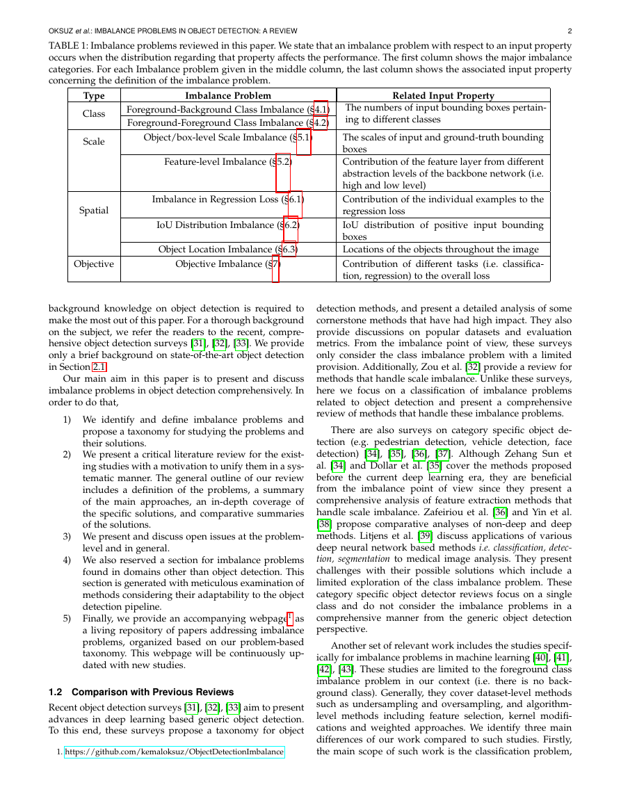
TABLE 1: Imbalance problems reviewed in this paper. We state that an imbalance problem with respect to an input property
occurs when the distribution regarding that property affects the performance. The first column shows the major imbalance
categories. For each Imbalance problem given in the middle column, the last column shows the associated input property
concerning the definition of the imbalance problem.
Imbalance Problem
Related Input Property
Type
Class
Scale
Spatial
Foreground-Background Class Imbalance (§4.1)
Foreground-Foreground Class Imbalance (§4.2)
Object/box-level Scale Imbalance (§5.1)
Feature-level Imbalance (§5.2)
Imbalance in Regression Loss (§6.1)
IoU Distribution Imbalance (§6.2)
Objective
Object Location Imbalance (§6.3)
Objective Imbalance (§7)
The numbers of input bounding boxes pertain-
ing to different classes
The scales of input and ground-truth bounding
boxes
Contribution of the feature layer from different
abstraction levels of the backbone network (i.e.
high and low level)
Contribution of the individual examples to the
regression loss
IoU distribution of positive input bounding
boxes
Locations of the objects throughout the image
Contribution of different tasks (i.e. classifica-
tion, regression) to the overall loss
background knowledge on object detection is required to
make the most out of this paper. For a thorough background
on the subject, we refer the readers to the recent, compre-
hensive object detection surveys [31], [32], [33]. We provide
only a brief background on state-of-the-art object detection
in Section 2.1.
Our main aim in this paper is to present and discuss
imbalance problems in object detection comprehensively. In
order to do that,
1) We identify and define imbalance problems and
propose a taxonomy for studying the problems and
their solutions.
2) We present a critical literature review for the exist-
ing studies with a motivation to unify them in a sys-
tematic manner. The general outline of our review
includes a definition of the problems, a summary
of the main approaches, an in-depth coverage of
the specific solutions, and comparative summaries
of the solutions.
3) We present and discuss open issues at the problem-
level and in general.
4) We also reserved a section for imbalance problems
found in domains other than object detection. This
section is generated with meticulous examination of
methods considering their adaptability to the object
detection pipeline.
Finally, we provide an accompanying webpage1 as
a living repository of papers addressing imbalance
problems, organized based on our problem-based
taxonomy. This webpage will be continuously up-
dated with new studies.
5)
1.2 Comparison with Previous Reviews
Recent object detection surveys [31], [32], [33] aim to present
advances in deep learning based generic object detection.
To this end, these surveys propose a taxonomy for object
1. https://github.com/kemaloksuz/ObjectDetectionImbalance
detection methods, and present a detailed analysis of some
cornerstone methods that have had high impact. They also
provide discussions on popular datasets and evaluation
metrics. From the imbalance point of view, these surveys
only consider the class imbalance problem with a limited
provision. Additionally, Zou et al. [32] provide a review for
methods that handle scale imbalance. Unlike these surveys,
here we focus on a classification of imbalance problems
related to object detection and present a comprehensive
review of methods that handle these imbalance problems.
There are also surveys on category specific object de-
tection (e.g. pedestrian detection, vehicle detection, face
detection) [34], [35], [36], [37]. Although Zehang Sun et
al. [34] and Dollar et al. [35] cover the methods proposed
before the current deep learning era, they are beneficial
from the imbalance point of view since they present a
comprehensive analysis of feature extraction methods that
handle scale imbalance. Zafeiriou et al. [36] and Yin et al.
[38] propose comparative analyses of non-deep and deep
methods. Litjens et al. [39] discuss applications of various
deep neural network based methods i.e. classification, detec-
tion, segmentation to medical image analysis. They present
challenges with their possible solutions which include a
limited exploration of the class imbalance problem. These
category specific object detector reviews focus on a single
class and do not consider the imbalance problems in a
comprehensive manner from the generic object detection
perspective.
Another set of relevant work includes the studies specif-
ically for imbalance problems in machine learning [40], [41],
[42], [43]. These studies are limited to the foreground class
imbalance problem in our context (i.e. there is no back-
ground class). Generally, they cover dataset-level methods
such as undersampling and oversampling, and algorithm-
level methods including feature selection, kernel modifi-
cations and weighted approaches. We identify three main
differences of our work compared to such studies. Firstly,
the main scope of such work is the classification problem,
�
OKSUZ et al.: IMBALANCE PROBLEMS IN OBJECT DETECTION: A REVIEW
which is still relevant for object detection; however, object
detection also has a “search” aspect, in addition to the
recognition aspect, which brings in the background (i.e.
negative) class into the picture. Secondly, except Johnson
et al. [43], they consider machine learning approaches in
general without any special focus on deep learning based
methods. Finally, and more importantly, these works only
consider foreground class imbalance problem, which is only
one of eight different imbalance problems that we present
and discuss here (Table 1).
1.3 A Guide to Reading This Review
The paper is organized as follows. Section 2 provides a brief
background on object detection, and the list of frequently-
used terms and notation used throughout the paper. Section
3 presents our taxonomy of imbalance problems. Sections 4-
7 then cover each imbalance problem in detail, with a critical
review of the proposed solutions and include open issues for
each imbalance problem. Each section dedicated to a specific
imbalance problem is designed to be self-readable, contain-
ing definitions and a review of the proposed methods. In
order to provide a more general perspective, in Section 8,
we present the solutions addressing imbalance in other but
closely related domains. Section 9 discusses open issues that
are relevant to all imbalance problems. Finally, Section 10
concludes the paper.
Readers who are familiar with the current state-of-the-art
object detection methods can directly jump to Section 3 and
use Figure 1 to navigate both the imbalance problems and
the sections dedicated to the different problems according to
the taxonomy. For readers who lack a background in state-
of-the-art object detection, we recommend starting with
Section 2.1, and if this brief background is not sufficient,
we refer the reader to the more in-depth reviews mentioned
in Section 1.1.
2 BACKGROUND, DEFINITIONS AND NOTATION
In the following, we first provide a brief background on
state-of-the-art object detection methods, and then present
the definitions and notations used throughout the paper.
2.1 State of the Art in Object Detection
Today there are two major approaches to object detection:
top-down and bottom-up. Although both the top-down
and bottom-up approaches were popular prior to the deep
learning era, today the majority of the object detection meth-
ods follow the top-down approach; the bottom-up methods
have been proposed relatively recently. The main difference
between the top-down and bottom-up approaches is that,
in the top-down approach, holistic object hypotheses (i.e.,
anchors, regions-of-interests/proposals) are generated and
evaluated early in the detection pipeline, whereas in the
bottom-up approach, holistic objects emerge by grouping
sub-object entities like keypoints or parts, later in the pro-
cessing pipeline.
Methods following the top-down approach are catego-
rized into two: two-stage and one-stage methods. Two-
stage methods [16], [17], [18], [21] aim to decrease the large
number of negative examples resulting from the predefined,
TABLE 2: Frequently used notations in the paper.
3
Symbol
B
C
|Ci|
Ci
I(P )
P i
pi
ps
p0
u
ˆx
Domain
See.Def.
A set of
integers
|Ci| ∈ Z+
i ∈ Z+
I(P ) ∈ {0, 1}
i ∈ Z+
pi ∈ [0, 1]
ps ∈ [0, 1]
p0 ∈ [0, 1]
u ∈ C
ˆx ∈ R
Denotes
A Bounding box
Set of Class labels in a dataset
Number of examples for the ith
class in a dataset
Backbone feature layer at depth i
Indicator function. 1 if predicate P
is true, else 0
Pyramidal feature layer
corresponding to ith backbone
feature layer
Confidence score of ith class (i.e.
output of classifier)
Confidence score of the ground
truth class
Confidence score of background
class
Class label of a ground truth
Input of the regression loss
dense sliding windows, called anchors, to a manageable
size by using a proposal mechanism [21], [44], [45] which
determines the regions where the objects most likely appear,
called Region of Interests (RoIs). These RoIs are further
processed by a detection network which outputs the object
detection results in the form of bounding boxes and associ-
ated object-category probabilities. Finally, the non-maxima
suppression (NMS) method is applied on the object de-
tection results to eliminate duplicate or highly-overlapping
results. NMS is a universal post-processing step used by all
state-of-the-art object detectors.
One-stage top-down methods, including SSD Variants
[19], [46], YOLO variants [15], [20], [47] and RetinaNet [22],
are designed to predict the detection results directly from
anchors – without any proposal elimination stage – after
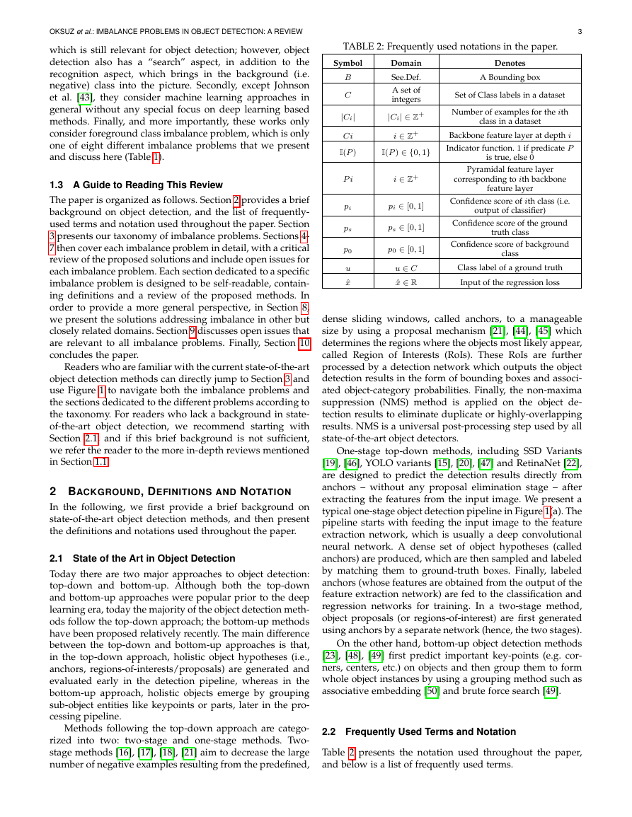
extracting the features from the input image. We present a
typical one-stage object detection pipeline in Figure 1(a). The
pipeline starts with feeding the input image to the feature
extraction network, which is usually a deep convolutional
neural network. A dense set of object hypotheses (called
anchors) are produced, which are then sampled and labeled
by matching them to ground-truth boxes. Finally, labeled
anchors (whose features are obtained from the output of the
feature extraction network) are fed to the classification and
regression networks for training. In a two-stage method,
object proposals (or regions-of-interest) are first generated
using anchors by a separate network (hence, the two stages).
On the other hand, bottom-up object detection methods
[23], [48], [49] first predict important key-points (e.g. cor-
ners, centers, etc.) on objects and then group them to form
whole object instances by using a grouping method such as
associative embedding [50] and brute force search [49].
2.2 Frequently Used Terms and Notation
Table 2 presents the notation used throughout the paper,
and below is a list of frequently used terms.
�
OKSUZ et al.: IMBALANCE PROBLEMS IN OBJECT DETECTION: A REVIEW
4
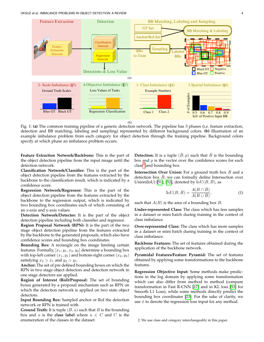
Fig. 1: (a) The common training pipeline of a generic detection network. The pipeline has 3 phases (i.e. feature extraction,
detection and BB matching, labeling and sampling) represented by different background colors. (b) Illustration of an
example imbalance problem from each category for object detection through the training pipeline. Background colors
specify at which phase an imbalance problem occurs.
Feature Extraction Network/Backbone: This is the part of
the object detection pipeline from the input image until the
detection network.
Classification Network/Classifier: This is the part of the
object detection pipeline from the features extracted by the
backbone to the classification result, which is indicated by a
confidence score.
Regression Network/Regressor: This is the part of the
object detection pipeline from the features extracted by the
backbone to the regression output, which is indicated by
two bounding box coordinates each of which consisting of
an x-axis and y-axis values.
Detection Network/Detector: It is the part of the object
detection pipeline including both classifier and regressor.
Region Proposal Network (RPN): It is the part of the two
stage object detection pipeline from the features extracted
by the backbone to the generated proposals, which also have
confidence scores and bounding box coordinates.
Bounding Box: A rectangle on the image limiting certain
features. Formally, [x1, y1, x2, y2] determine a bounding box
with top-left corner (x1, y1) and bottom-right corner (x2, y2)
satisfying x2 > x1 and y2 > y1.
Anchor: The set of pre defined bounding boxes on which the
RPN in two stage object detectors and detection network in
one stage detectors are applied.
Region of Interest (RoI)/Proposal: The set of bounding
boxes generated by a proposal mechanism such as RPN on
which the detection network is applied on two state object
detectors.
Input Bounding Box: Sampled anchor or RoI the detection
network or RPN is trained with.
Ground Truth: It is tuple (B, u) such that B is the bounding
box and u is the class label where u ∈ C and C is the
enumeration of the classes in the dataset.
Detection: It is a tuple ( ¯B, p) such that ¯B is the bounding
box and p is the vector over the confidence scores for each
class2 and bounding box.
Intersection Over Union: For a ground truth box B and a
detection box ¯B, we can formally define Intersection over
Union(IoU) [51], [52], denoted by IoU(B, ¯B), as
A(B ∩ ¯B)
A(B ∪ ¯B)
IoU(B, ¯B) =
,
(1)
such that A(B) is the area of a bounding box B.
Under-represented Class: The class which has less samples
in a dataset or mini batch during training in the context of
class imbalance.
Over-represented Class: The class which has more samples
in a dataset or mini batch during training in the context of
class imbalance.
Backbone Features: The set of features obtained during the
application of the backbone network.
Pyramidal Features/Feature Pyramid: The set of features
obtained by applying some transformations to the backbone
features.
Regression Objective Input: Some methods make predic-
tions in the log domain by applying some transformation
which can also differ from method to method (compare
transformation in Fast R-CNN [17] and in KL loss [53] for
Smooth L1 Loss), while some methods directly predict the
bounding box coordinates [23]. For the sake of clarity, we
use ˆx to denote the regression loss input for any method.
2. We use class and category interchangeably in this paper.
BB Matching & LabelingAnchor/RoISetGT SetFeature ExtractionDetectionBB Matching, Labeling and SamplingBlue GTBlack GTPositiveNegativeSamplingGround Truth Scales2-Scale Imbalance(§5)Loss Values of Tasks4-ObjectiveImbalance(§7)1-Class Imbalance(§4)Class 1Class 23-SpatialImbalance(§6)IoUof Positive Input BB0.60.50.70.80.9# of ExamplesDetections & Loss ValueClassificationRegressionBBstoTrainLabeledBBs(a)(b)Example NumbersBlack GTBlue GTFeature Extraction Network�
OKSUZ et al.: IMBALANCE PROBLEMS IN OBJECT DETECTION: A REVIEW
5
• See generative methods for
fg-bg class imb.
• Fine-tuning Long Tail
Distribution for Obj.Det. [25]
• OFB Sampling [66]
Fg-Fg Class
Imbalance
(§4.2)
Fg-Bg Class
Imbalance
(§4.1)
Object/box-
level Imbalance
(§5.1)
Class Imbalance
(§4)
• Task Weighting
• Classification Aware
Regression Loss [30]
• Guided Loss [54]
Objective Imbalance
(§7)
Methods for
Imbalance Problems
Scale Imbalance
(§5)
Feature-level
Imbalance
(§5.2)
Imbalance in
Regression Task
(§6.1)
Spatial Imbalance
(§6)
Object
Location
Imbalance
(§6.3)
•1.Hard Sampling Methods
• A.Random Sampling
• B.Hard Example Mining
– Bootstraping [55]
– SSD [19]
– Online Hard Example Mining [24]
– IoU-based Sampling [29]
• C.Limit Search Space
– Two-stage Object Detectors
– IoU-lower Bound [17]
– Objectness Prior [56]
– Negative Anchor Filtering [57]
– Objectness Module [58]
•2.Soft Sampling Methods
• Focal Loss [22]
• Gradient Harmonizing Mechanism [59]
• Prime Sample Attention [30]
•3.Sampling-Free Methods
• Residual Objectness [60]
• No Sampling Heuristics [54]
• AP Loss [61]
• DR Loss [62]
•4.Generative Methods
• Adversarial Faster-RCNN [63]
• Task Aware Data Synthesis [64]
• PSIS [65]
• pRoI Generator [66]
•1.Methods Predicting from the Feature Hierarchy of
Backbone Features
• Scale-dependent Pooling [69]
• SSD [19]
• Multi Scale CNN [70]
• Scale Aware Fast R-CNN [71]
•2.Methods Based on Feature Pyramids
• FPN [26]
• See feature-level imbalance methods
•3.Methods Based on Image Pyramids
• SNIP [27]
• SNIPER [28]
•4.Methods Combining Image and Feature Pyramids
• Efficient Featurized Image Pyramids [72]
• Enriched Feature Guided Refinement Network [58]
• Super Resolution for Small Objects [73]
• Scale Aware Trident Network [74]
•1.Lp norm based
• Smooth L1 [17]
• Balanced L1 [29]
• KL Loss [53]
• Gradient Harmonizing
Mechanism [59]
•2.IoU based
• IoU Loss [83]
• Bounded IoU Loss [84]
• GIoU Loss [85]
• Distance IoU Loss [86]
• Complete IoU Loss [86]
IoU
Distribution
Imbalance
(§6.2)
• Guided Anchoring [67]
• Free Anchor [68]
• Cascade R-CNN [87]
• HSD [88]
• IoU-uniform R-CNN [89]
• pRoI Generator [66]
•1.Methods Using Pyramidal Features as a Basis
• PANet [75]
• Libra FPN [29]
•2.Methods Using Backbone Features as a Basis
• STDN [76]
• Parallel-FPN [77]
• Deep Feature Pyramid Reconf. [78]
• Zoom Out-and-In [79]
• Multi-level FPN [80]
• NAS-FPN [81]
• Auto-FPN [82]
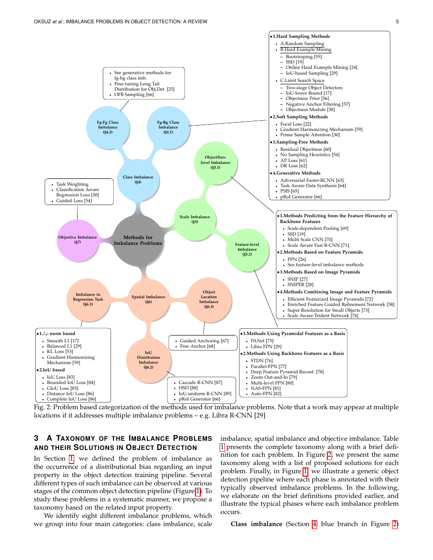
Fig. 2: Problem based categorization of the methods used for imbalance problems. Note that a work may appear at multiple
locations if it addresses multiple imbalance problems – e.g. Libra R-CNN [29]
3 A TAXONOMY OF THE IMBALANCE PROBLEMS
AND THEIR SOLUTIONS IN OBJECT DETECTION
In Section 1, we defined the problem of imbalance as
the occurrence of a distributional bias regarding an input
property in the object detection training pipeline. Several
different types of such imbalance can be observed at various
stages of the common object detection pipeline (Figure 1). To
study these problems in a systematic manner, we propose a
taxonomy based on the related input property.
We identify eight different imbalance problems, which
we group into four main categories: class imbalance, scale
imbalance, spatial imbalance and objective imbalance. Table
1 presents the complete taxonomy along with a brief defi-
nition for each problem. In Figure 2, we present the same
taxonomy along with a list of proposed solutions for each
problem. Finally, in Figure 1, we illustrate a generic object
detection pipeline where each phase is annotated with their
typically observed imbalance problems. In the following,
we elaborate on the brief definitions provided earlier, and
illustrate the typical phases where each imbalance problem
occurs.
Class imbalance (Section 4; blue branch in Figure 2)
�
OKSUZ et al.: IMBALANCE PROBLEMS IN OBJECT DETECTION: A REVIEW
6
occurs when a certain class is over-represented. This prob-
lem can manifest itself as either “foreground-background
imbalance,” where the background instances significantly
outnumber the positive ones; or “foreground-foreground
imbalance,” where typically a small fraction of classes dom-
inate the dataset (as observed from the long-tail distribution
in Figure 5). The class imbalance is usually handled at the
“sampling” stage in the object detection pipeline (Figure 1).
Scale imbalance (Section 5; green branch in Figure 2)
is observed when object instances have various scales and
different number of examples pertaining to different scales.
This problem is a natural outcome of the fact that objects
have different dimensions in nature. Scale also could cause
imbalance at the feature-level (typically handled in the
“feature extraction” phase in Figure 1), where contribution
from different abstraction layers (i.e. high and low levels)
are not balanced. Scale imbalance problem suggests that a
single scale of visual processing is not sufficient for detect-
ing objects at different scales. However, as we will see in
Section 5, proposed methods fall short in addressing scale
imbalance, especially for small objects, even when small
objects are surprisingly abundant in a dataset.
Spatial imbalance (Section 6; orange branch in Figure
2) refers to a set of factors related to spatial properties of
the bounding boxes. Owing to these spatial properties, we
identify three sub-types of spatial imbalance: (i) “imbalance
in regression loss” is about the contributions of individual
examples to the regression loss and naturally the problem
is related to loss function design (ii) “IoU distribution im-
balance” is related to the biases in the distribution of IoUs
(among ground-truth boxes vs. anchors or detected boxes),
and typically observed at the bounding-box matching and
labeling phase in the object detection pipeline (Figure 1) (iii)
“object location imbalance” is about the location distribution
of object instances in an image, which is related to both the
design of the anchors and the sampled subset to train the
detection network.
Finally, objective imbalance (Section 7; purple branch
in Figure 2) occurs when there are multiple objectives (loss
functions) to minimize (each for a specific task, e.g. classifi-
cation and box-regression). Since different objectives might
be incompatible in terms of their ranges as well as their
optimum solutions, it is essential to develop a balanced
strategy that can find a solution acceptable in terms of all
objectives.
Figure 2 gives an overall picture of the attention that
different types of imbalance problems have received from
the research community. For example, while there are nu-
merous methods devised for the foreground-background
class imbalance problem, the objective imbalance and object
location imbalance problems are examples of the problems
that received relatively little attention. However, recently
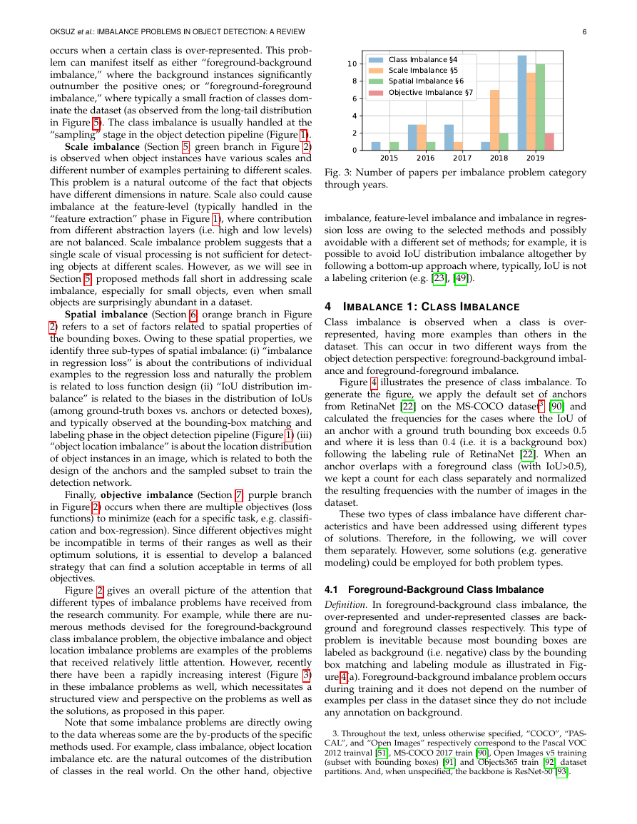
there have been a rapidly increasing interest (Figure 3)
in these imbalance problems as well, which necessitates a
structured view and perspective on the problems as well as
the solutions, as proposed in this paper.
Note that some imbalance problems are directly owing
to the data whereas some are the by-products of the specific
methods used. For example, class imbalance, object location
imbalance etc. are the natural outcomes of the distribution
of classes in the real world. On the other hand, objective
Fig. 3: Number of papers per imbalance problem category
through years.
imbalance, feature-level imbalance and imbalance in regres-
sion loss are owing to the selected methods and possibly
avoidable with a different set of methods; for example, it is
possible to avoid IoU distribution imbalance altogether by
following a bottom-up approach where, typically, IoU is not
a labeling criterion (e.g. [23], [49]).
imbalance is observed when a class
4 IMBALANCE 1: CLASS IMBALANCE
Class
is over-
represented, having more examples than others in the
dataset. This can occur in two different ways from the
object detection perspective: foreground-background imbal-
ance and foreground-foreground imbalance.
Figure 4 illustrates the presence of class imbalance. To
generate the figure, we apply the default set of anchors
from RetinaNet [22] on the MS-COCO dataset3 [90] and
calculated the frequencies for the cases where the IoU of
an anchor with a ground truth bounding box exceeds 0.5
and where it is less than 0.4 (i.e. it is a background box)
following the labeling rule of RetinaNet [22]. When an
anchor overlaps with a foreground class (with IoU>0.5),
we kept a count for each class separately and normalized
the resulting frequencies with the number of images in the
dataset.
These two types of class imbalance have different char-
acteristics and have been addressed using different types
of solutions. Therefore, in the following, we will cover
them separately. However, some solutions (e.g. generative
modeling) could be employed for both problem types.
4.1 Foreground-Background Class Imbalance
Definition. In foreground-background class imbalance, the
over-represented and under-represented classes are back-
ground and foreground classes respectively. This type of
problem is inevitable because most bounding boxes are
labeled as background (i.e. negative) class by the bounding
box matching and labeling module as illustrated in Fig-
ure 4(a). Foreground-background imbalance problem occurs
during training and it does not depend on the number of
examples per class in the dataset since they do not include
any annotation on background.
3. Throughout the text, unless otherwise specified, “COCO”, “PAS-
CAL”, and “Open Images” respectively correspond to the Pascal VOC
2012 trainval [51], MS-COCO 2017 train [90], Open Images v5 training
(subset with bounding boxes) [91] and Objects365 train [92] dataset
partitions. And, when unspecified, the backbone is ResNet-50 [93].
201520162017201820190246810Class Imbalance §4Scale Imbalance §5Spatial Imbalance §6Objective Imbalance §7�
OKSUZ et al.: IMBALANCE PROBLEMS IN OBJECT DETECTION: A REVIEW
7
(a)
(b)
Fig. 4: Illustration of the class imbalance problems. The numbers of RetinaNet [22] anchors on MS-COCO [90] are plotted
for foreground-background (a), and foreground classes (b). The values are normalized with the total number of images in
the dataset. The figures depict severe imbalance towards some classes.
Solutions. We can group the solutions for the foreground-
background class imbalance into four: (i) hard sampling
methods, (ii) soft sampling methods, (iii) sampling-free
methods and (iv) generative methods. Each set of methods
are explained in detail in the subsections below.
In sampling methods, the contribution (wi) of a bound-
ing box (BBi) to the loss function is adjusted as follows:
wiCE(ps),
(2)
where CE() is the cross-entropy loss. Hard and soft sam-
pling approaches differ on the possible values of wi. For
the hard sampling approaches, wi ∈ {0, 1}, thus a BB is
either selected or discarded. For soft sampling approaches,
wi ∈ [0, 1], i.e. the contribution of a sample is adjusted with
a weight and each BB is somehow included in training.
4.1.1 Hard Sampling Methods
Hard sampling is a commonly-used method for addressing
imbalance in object detection. It restricts wi to be binary; i.e.,
0 or 1. In other words, it addresses imbalance by selecting
a subset of positive and negative examples (with desired
quantities) from a given set of labeled BBs. This selection
is performed using heuristic methods and the non-selected
examples are ignored for the current iteration. Therefore,
each sampled example contributes equally to the loss (i.e.
wi = 1) and the non-selected examples (wi = 0) have no
contribution to the training for the current iteration. See
Table 3 for a summary of the main approaches.
A straightforward hard-sampling method is random
sampling. Despite its simplicity, it is employed in R-CNN
family of detectors [16], [21] where, for training RPN, 128
positive examples are sampled uniformly at random (out
of all positive examples) and 128 negative anchors are
sampled in a similar fashion; and 16 positive examples and
48 negative RoIs are sampled uniformly from each image
in the batch at random from within their respective sets,
for training the detection network [17]. In any case, if the
number of positive input bounding boxes is less than the
desired values, the mini-batch is padded with randomly
sampled negatives. On the other hand, it has been reported
that other sampling strategies may perform better when a
property of an input box such as its loss value or IoU is
taken into account [24], [29], [30].
The first set of approaches to consider a property of
the sampled examples, rather than random sampling, is
the Hard-example mining methods4. These methods rely
on the hypothesis that training a detector more with hard
examples (i.e. examples with high losses) leads to better
performance. The origins of this hypothesis go back to the
bootstrapping idea in the early works on face detection [55],
[94], [95], human detection [96] and object detection [13].
The idea is based on training an initial model using a subset
of negative examples, then using the negative examples on
which the classifier fails (i.e. hard examples), a new classifier
is trained. Multiple classifiers are obtained by applying the
same procedure iteratively. Currently deep-learning-based
methods also adopt some versions of the hard example min-
ing in order to provide more useful examples by using the
loss values of the examples. The first deep object detector to
use hard examples in the training was Single-Shot Detector
[19], which chooses only the negative examples incurring
the highest loss values. A more systematic approach con-
sidering the loss values of positive and negative samples
is proposed in Online Hard Example Mining (OHEM) [24].
However, OHEM needs additional memory and causes the
training speed to decrease. Considering the efficiency and
memory problems of OHEM, IoU-based sampling [29] was
proposed to associate the hardness of the examples with
their IoUs and to use a sampling method again for only
negative examples rather than computing the loss function
for the entire set. In the IoU-based sampling, the IoU interval
for the negative samples is divided into K bins and equal
number of negative examples are sampled randomly within
each bin to promote the samples with higher IoUs, which
are expected to have higher loss values.
To improve mining performance, several studies pro-
posed to limit the search space in order to make hard
examples easy to mine. Two-stage object detectors [18], [21]
are among these methods since they aim to find the most
probable bounding boxes (i.e. RoIs) given anchors, and then
choose top N RoIs with the highest objectness scores, to
which an additional sampling method is applied. Fast R-
CNN [17] sets the lower bound of IoU of the negative RoIs
4. In this paper, we adopt the boldface font whenever we introduce
an approach involving a set of different methods, and the method
names themselves are in italic.
Number of Anchors for Bg and Fg166827.50 163.04BackgroundForegroundClasses00.511.52Number of Anchors105Number of Anchors for Fg Classes01020304050607080Foreground Classes01020304050Number of Anchors�
OKSUZ et al.: IMBALANCE PROBLEMS IN OBJECT DETECTION: A REVIEW
to 0.1 rather than 0 for promoting hard negatives and
then applies random sampling. Kong et al. [56] proposed a
method that learns objectness priors in an end-to-end setting
in order to have a guidance on where to search for the
objects. All of the positive examples having an objectness
prior larger than a threshold are used during training, while
the negative examples are selected such that the desired
balance (i.e. 1 : 3) is preserved between positive and neg-
ative classes. Zhang et al. [57] proposed determining the
confidence scores of anchors with the anchor refinement
module in a one-stage detection pipeline and again adopted
a threshold to eliminate the easy negative anchors. The
authors coined their approach as negative anchor filtering.
Nie et al. [58] used a cascaded-detection scheme in the SSD
pipeline which includes an Objectness Module before each
prediction module. These objectness modules are binary
classifiers to filter out the easy anchors.
4.1.2 Soft Sampling Methods
Soft sampling adjusts the contribution (wi) of each example
by its relative importance to the training process. This way,
unlike hard sampling, no sample is discarded and the whole
dataset is utilized for updating the parameters. See Table 3
for a summary of the main approaches.
A straightforward approach is to use constant coeffi-
cients for both the foreground and background classes.
YOLO [20], having less number of anchors compared to
other one-stage methods such as SSD [19] and RetinaNet
[22], is a straightforward example for soft sampling in which
the loss values of the examples from the background class
are halved (i.e. wi = 0.5).
Focal Loss [22] is the pioneer example that dynamically
assigns more weight to the hard examples as follows:
wi = (1 − ps)γ,
(3)
where ps is the estimated probability for the ground-truth
class. Since lower ps implies a larger error, Equation (3)
promotes harder examples. Note that when γ = 0, focal
loss degenerates to vanilla cross entropy loss and Lin et al.
[22] showed that γ = 2 ensures a good trade-off between
hard and easy examples for their architecture.
Similar to focal loss [22], Gradient Harmonizing Mech-
anism (GHM) [59] suppresses gradients originating from
easy positives and negatives. The authors first observed that
there are too many samples with small gradient norm, only
limited number of samples with medium gradient norm and
significantly large amount of samples with large gradient
norm. Unlike focal loss, GHM is a counting-based approach
which counts the number of examples with similar gradient
norm and penalizes the loss of a sample if there are many
samples with similar gradients as follows:
wi =
1
G(BBi)/m
,
(4)
where G(BBi) is the count of samples whose gradient norm
is close to the gradient norm of BBi; and m is the number
of input bounding boxes in the batch. In this sense, the
GHM method implicitly assumes that easy examples are
those with too many similar gradients. Different from other
methods, GHM is shown to be useful not only for classifica-
tion task but also for the regression task. In addition, since
the purpose is to balance the gradients within each task, this
method is also relevant to the “imbalance in regression loss”
discussed in Section 6.1.
8
Different from the latter soft sampling methods, PrIme
Sample Attention (PISA) [30] assigns weights to positive and
negative examples based on different criteria. While the
positive ones with higher IoUs are favored, the negatives
with larger foreground classification scores are promoted.
More specifically, PISA first ranks the examples for each
class based on their desired property (IoU or classification
score) and calculates a normalized rank, ¯ri, for each example
i as follows:
Nmax − ri
,
¯ri =
Nmax
(5)
where ri (0 ≤ ri ≤ Nj−1) is the rank of the ith example and
Nmax is the maximum number of examples over all classes
in the batch. Based on the normalized rank, the weight of
each example is defined as:
wi = ((1 − β)¯ri + β)γ,
(6)
where β adjusts the contribution of the normalized rank
and hence, the minimum sample weight; and γ is the
modulating factor again. These parameters are validated
for positives and negatives independently. Note that the
balancing strategy in Equations (5) and (6) increases the
contribution of the samples with high IoUs for positives and
high scores for negatives to the loss.
4.1.3 Sampling-Free Methods
Recently, alternative methods emerged in order to avoid
the aforementioned hand-crafted sampling heuristics and
therefore, decrease the number of hyperparameters during
training. For this purpose, Chen et al. [60] added an ob-
jectness branch to the detection network in order to predict
Residual Objectness scores. While this new branch tackles the
foreground-background imbalance, the classification branch
handles only the positive classes. During inference, clas-
sification scores are obtained by multiplying classification
and objectness branch outputs. The authors showed that
such a cascaded pipeline improves the performance. This
architecture is trained using vanilla cross entropy loss.
Another recent approach [54] suggests that if the hy-
perparameters are set appropriately, not only the detector
can be trained without any sampling mechanism but also
the performance can be improved. Accordingly, the authors
propose methods for setting the initialization bias,
loss
weighting (see Section 7) and class-adaptive threshold, and
in such a way they trained the network using vanilla cross
entropy loss achieving better performance.
Finally, an alternative method is to directly model the
final performance measure and weigh examples based on
this model. This approach is adopted by AP Loss [61] which
formulates the classification part of the loss as a ranking task
(see also DR Loss [62] which also uses a ranking method to
define a classification loss based on Hinge Loss) and uses
average precision (AP) as the loss function for this task. In
this method, the confidence scores are first transformed as
xij = −(pi − pj) such that pi is the confidence score of the
ith bounding box. Then, based on the transformed values,
�




 2023年江西萍乡中考道德与法治真题及答案.doc
 2012年重庆南川中考生物真题及答案.doc
 2013年江西师范大学地理学综合及文艺理论基础考研真题.doc
 2020年四川甘孜小升初语文真题及答案I卷.doc
 2020年注册岩土工程师专业基础考试真题及答案.doc
 2023-2024学年福建省厦门市九年级上学期数学月考试题及答案.doc
 2021-2022学年辽宁省沈阳市大东区九年级上学期语文期末试题及答案.doc
 2022-2023学年北京东城区初三第一学期物理期末试卷及答案.doc
 2018上半年江西教师资格初中地理学科知识与教学能力真题及答案.doc
 2012年河北国家公务员申论考试真题及答案-省级.doc
 2020-2021学年江苏省扬州市江都区邵樊片九年级上学期数学第一次质量检测试题及答案.doc
 2022下半年黑龙江教师资格证中学综合素质真题及答案.doc