Maximum Likelihood Programming in
Stata
Marco R. Steenbergen
Department of Political Science
University of North Carolina, Chapel Hill
August 2003
Contents
1 Introduction
2 Features
2
2
3 Syntactic Structure
2
3
3.1 Program Instructions . . . . . . . . . . . . . . . . . . . . . . . . . . . . . . . . .
6
. . . . . . . . . . . . . . . . . . . . . . . . . . . . . . . . . . . . . . .
3.2 Ml Model
6
3.2.1 Equations . . . . . . . . . . . . . . . . . . . . . . . . . . . . . . . . . . .
7
3.2.2 Additional Examples . . . . . . . . . . . . . . . . . . . . . . . . . . . . .
8
3.2.3 Options . . . . . . . . . . . . . . . . . . . . . . . . . . . . . . . . . . . .
8
3.3 Ml Check . . . . . . . . . . . . . . . . . . . . . . . . . . . . . . . . . . . . . . .
8
3.4 Ml Search . . . . . . . . . . . . . . . . . . . . . . . . . . . . . . . . . . . . . . .
3.5 Ml Maximize . . . . . . . . . . . . . . . . . . . . . . . . . . . . . . . . . . . . .
9
3.6 Monitoring Convergence and Ml Graph . . . . . . . . . . . . . . . . . . . . . . 10
4 Output
5 Performing Wald Tests
6 Performing Likelihood Ratio Tests
7 General Programming Issues
8 Additional MLE Features in Stata 8
9 References
10
12
13
15
15
17
1
�
1
Introduction
Maximum likelihood-based methods are now so common that most statistical
software packages have “canned” routines for many of those methods. Thus, it
is rare that you will have to program a maximum likelihood estimator yourself.
However, if this need arises (for example, because you are developing a new
method or want to modify an existing one), then Stata offers a user-friendly
and flexible programming language for maximum likelihood estimation (MLE).
In this document, I describe the basic syntax elements that allow you to
write and execute MLE routines in Stata (Versions 7 and 8). I do not intend to
offer an in-depth discussion of all of Stata’s many features—for this you should
consult Gould and Sribney (1999) and Gould, Pitblado, and Sribney (2003).
My objective is merely to provide you with enough tools that you can write a
simple MLE program and implement it.
2 Features
Stata has many nice features, including: (1) quick convergence (under most
circumstances) using the Newton-Raphson algorithm (Stata 8 also offers quasi-
Newton algorithms); (2) a conservative approach to declaring convergence, which
leads to more trustworthy estimates; (3) simplifying features that allow imple-
menting MLE with a minimum of calculus; (4) robust variance estimation; (5)
Wald and likelihood ratio test procedures; (6) a search routine that chooses
improved starting values; (7) estimation under linear constraints; and (8) post-
estimation commands. These features make Stata one of the easiest MLE pro-
grams to work with.
3 Syntactic Structure
Programming and executing MLE routines in Stata requires a specific sequence
of commands. These may be part of an ado file, or they can be entered in-
teractively. The following shows the sequence of commands and explains their
meaning. Optional commands are indicated by an asterisk.
1. Program instructions: The program specifies the parameters and log-
likelihood function. This is done in general terms, so that the commands
can be used in any application where they are relevant. (The program
may be kept in a separate ado file.)
2. ml model:1 This command specifies the model that is to be estimated
(i.e., dependent variable and predictors), as well as the MLE program
that should be run and the way in which it should be run. This command
is application-specific: it specifies the model in terms of the particular set
of variables that is loaded into memory.
1In this document, I indicate Stata commands in print type.
2
�
3. ml check*: This command checks the program syntax for mistakes. While
optional, it is extremely useful for debugging MLE routines. Beginning
programmers are advised to use this command.
4. ml search*: This optional command causes Stata to search for better
starting values for the numerical optimization algorithm.
5. ml maximize: This command starts the execution of the estimation com-
mands and generates the output.
6. ml graph*: This is an optional command that produces a graph showing
the iteration path of the numerical optimization algorithm. I recommend
using this command so that one can monitor convergence.
3.1 Program Instructions
In most cases, writing and MLE program requires only a couple of lines of
syntax. At least, this is the case if (1) the log-likelihood function meets the
linear form restriction—i.e., the observations are independent—and (2) Stata
derives the first and second (partial) derivatives numerically (these derivatives
are needed for the Newton-Raphson algorithm).
In this document, I assume
that these two conditions are met.2
The program is started by entering
program define name
where name is any name up to 32 characters in length.
(It is preferable to
choose a descriptive name.) The user may abbreviate program define to pr
de. To end the program, one should type
end
In between these keywords, the user has to declare the parameters and the
log-likelihood function. First, the log-likelihood function and its parameters
have to be labeled. This is done through the command args (which is an
abbreviation for the computer term “arguments”). Next, the log-likelihood
function has to be defined; this is done using the quietly replace command.3
In addition to these specifications, it is often useful to declare the program
version, especially if you are planning to make changes to the program over
time.
2That is, the maximization method is lf (see the discussion of ml model below). Please
note that lf is the easiest approach in Stata but not always the most accurate. However, in
my programming experience I have never encountered an instance in which the results from
lf were misleading.
3“Replace” indicates that the user is substituting a new expression. “Quietly” implies that
Stata does not echo this substitution—i.e., it is not displayed on the screen or in the output.
3
�
Example 1: To show the use of these commands, consider the simple example
of the Poisson distribution:
f(y|µ) = µye−µ
y!
ln(yi!)
Here µ is the parameter that we want to estimate. For a sample of n independent
observations, this distribution produces the following log-likelihood function:
l(µ|y1, y2 ··· yn) =
yi ln(µ) − nµ −
To program this function, we could use the following syntax:
i
i
program define poisson
version 1.0
args lnf mu
quietly replace ‘lnf’ = $ML y1*ln(‘mu’)- ‘mu’ - lnfact($ML y1)
end
Let us analyze what this program does. In the first line we define the pro-
gram, calling it poisson. In the second line, we show the version of the program
(version 1.0). The third line provides a name for the log-likelihood function
(lnf) and its one parameter (mu). The fourth line specifies the log-likelihood
function and the fifth line ends the program.
The action, of course, is in the fourth line. This line is based on the argu-
ments specified in args. Because we are referring to arguments, they should
be placed in apostrophes. (In fact, the leading apostrophe is backward leaning
and is typically located on the same key as the tilde; the second apostrophe
is straight and is typically located on the same key as the double apostrophe.)
The fourth line also contains the variable $ML y1, which is the internal label
for the (first) dependent variable. Stata will replace this with an appropriate
variable from the data set after the ml model command has been specified.4
Finally, the fourth line specifies a function. (The last term in this expression,
lnfact($ML y1), stands for ln(y!).)
A careful inspection of the fourth line of code shows that it looks a lot like
the log-likelihood function, except that it does not include summations. In fact,
this line gives the log-likelihood function for a single observation:
l(µ|yi) = yi ln(µ) − µ − ln(yi!)
As long as the observations are independent (i.e., the linear form restriction on
the log-likelihood function is met), this is all you have to specify. Stata knows
that it should evaluate this function for each observation in the data and then
sum the results. This greatly simplifies programming log-likelihood functions.5
4By not referring to a specific variable name, the program can be used for any data set.
This is quite useful, as you do not have to go back into the program to change variable names.
5Keep in mind, however, that this will only work if the observations are independent and
the linear form restriction is met.
4
�
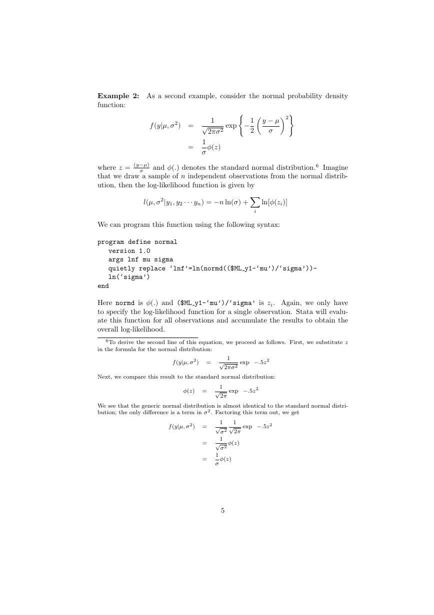
Example 2: As a second example, consider the normal probability density
function:
2
−1
2
y − µ
σ
f(y|µ, σ2) =
=
exp
1√
2πσ2
1
σ
φ(z)
σ
where z = (y−µ)
and φ(.) denotes the standard normal distribution.6 Imagine
that we draw a sample of n independent observations from the normal distrib-
ution, then the log-likelihood function is given by
l(µ, σ2|y1, y2 ··· yn) = −n ln(σ) +
ln[φ(zi)]
We can program this function using the following syntax:
i
program define normal
version 1.0
args lnf mu sigma
quietly replace ‘lnf’=ln(normd(($ML y1-‘mu’)/‘sigma’))-
ln(‘sigma’)
end
Here normd is φ(.) and ($ML y1-‘mu’)/‘sigma’ is zi. Again, we only have
to specify the log-likelihood function for a single observation. Stata will evalu-
ate this function for all observations and accumulate the results to obtain the
overall log-likelihood.
6To derive the second line of this equation, we proceed as follows. First, we substitute z
in the formula for the normal distribution:
f (y|µ, σ2) =
1√
2πσ2
Next, we compare this result to the standard normal distribution:
We see that the generic normal distribution is almost identical to the standard normal distri-
bution; the only difference is a term in σ2. Factoring this term out, we get
exp
−.5z2
−.5z2
−.5z2
φ(z) =
1√
2π
exp
f (y|µ, σ2) =
=
=
exp
1√
2π
φ(z)
1√
σ2
1√
σ2
1
σ
φ(z)
5
�
3.2 Ml Model
To apply a program to a data set, you need to issue the ml model command.
This command also controls the method of maximization that is used, but I will
assume that this method is lf—i.e., the linear form restrictions hold and the
derivatives are obtained numerically.7
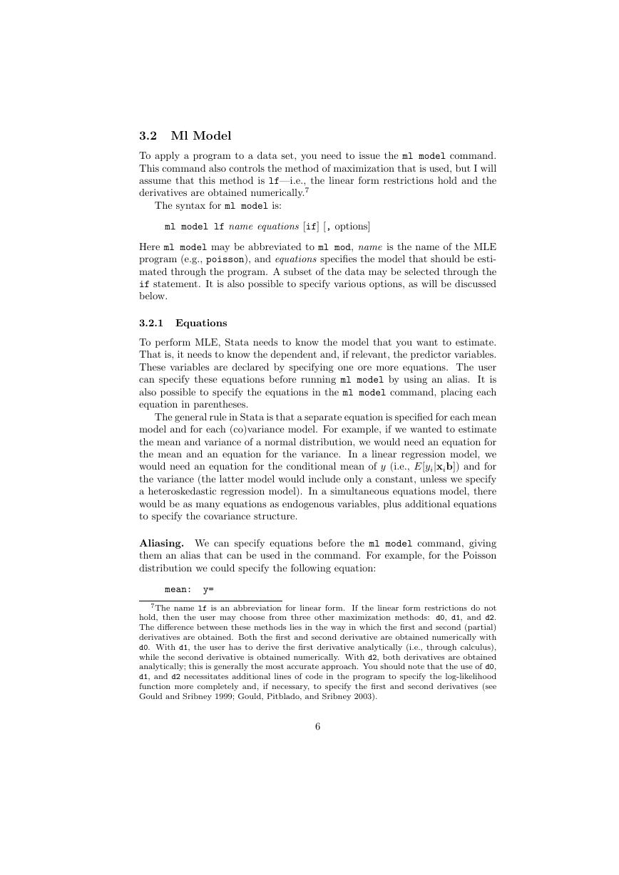
The syntax for ml model is:
ml model lf name equations [if] [, options]
Here ml model may be abbreviated to ml mod, name is the name of the MLE
program (e.g., poisson), and equations specifies the model that should be esti-
mated through the program. A subset of the data may be selected through the
if statement. It is also possible to specify various options, as will be discussed
below.
3.2.1 Equations
To perform MLE, Stata needs to know the model that you want to estimate.
That is, it needs to know the dependent and, if relevant, the predictor variables.
These variables are declared by specifying one ore more equations. The user
can specify these equations before running ml model by using an alias. It is
also possible to specify the equations in the ml model command, placing each
equation in parentheses.
The general rule in Stata is that a separate equation is specified for each mean
model and for each (co)variance model. For example, if we wanted to estimate
the mean and variance of a normal distribution, we would need an equation for
the mean and an equation for the variance. In a linear regression model, we
would need an equation for the conditional mean of y (i.e., E[yi|xib]) and for
the variance (the latter model would include only a constant, unless we specify
a heteroskedastic regression model). In a simultaneous equations model, there
would be as many equations as endogenous variables, plus additional equations
to specify the covariance structure.
Aliasing. We can specify equations before the ml model command, giving
them an alias that can be used in the command. For example, for the Poisson
distribution we could specify the following equation:
mean:
y=
7The name lf is an abbreviation for linear form.
If the linear form restrictions do not
hold, then the user may choose from three other maximization methods: d0, d1, and d2.
The difference between these methods lies in the way in which the first and second (partial)
derivatives are obtained. Both the first and second derivative are obtained numerically with
d0. With d1, the user has to derive the first derivative analytically (i.e., through calculus),
while the second derivative is obtained numerically. With d2, both derivatives are obtained
analytically; this is generally the most accurate approach. You should note that the use of d0,
d1, and d2 necessitates additional lines of code in the program to specify the log-likelihood
function more completely and, if necessary, to specify the first and second derivatives (see
Gould and Sribney 1999; Gould, Pitblado, and Sribney 2003).
6
�
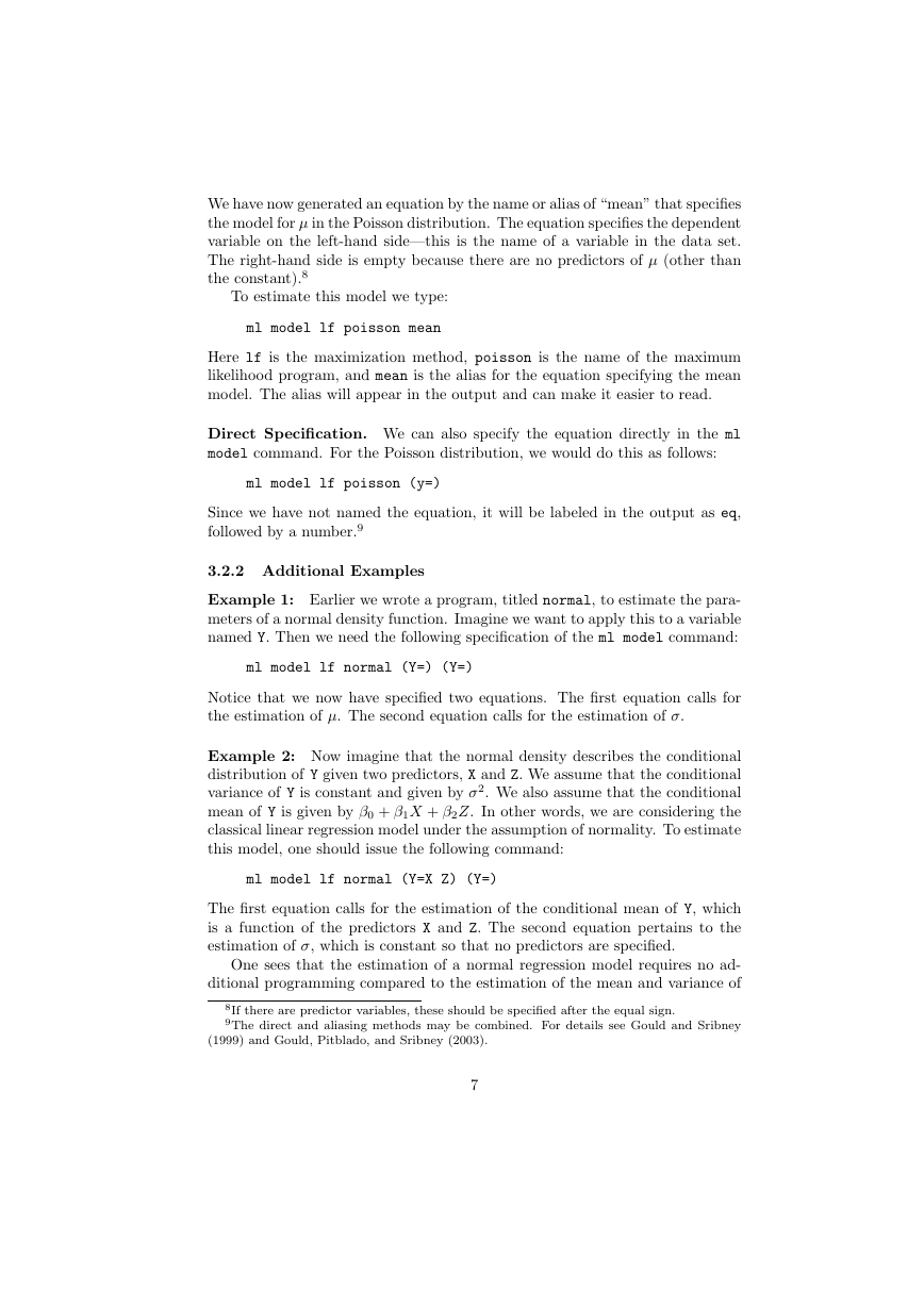
We have now generated an equation by the name or alias of “mean” that specifies
the model for µ in the Poisson distribution. The equation specifies the dependent
variable on the left-hand side—this is the name of a variable in the data set.
The right-hand side is empty because there are no predictors of µ (other than
the constant).8
To estimate this model we type:
ml model lf poisson mean
Here lf is the maximization method, poisson is the name of the maximum
likelihood program, and mean is the alias for the equation specifying the mean
model. The alias will appear in the output and can make it easier to read.
Direct Specification. We can also specify the equation directly in the ml
model command. For the Poisson distribution, we would do this as follows:
ml model lf poisson (y=)
Since we have not named the equation, it will be labeled in the output as eq,
followed by a number.9
3.2.2 Additional Examples
Example 1: Earlier we wrote a program, titled normal, to estimate the para-
meters of a normal density function. Imagine we want to apply this to a variable
named Y. Then we need the following specification of the ml model command:
ml model lf normal (Y=) (Y=)
Notice that we now have specified two equations. The first equation calls for
the estimation of µ. The second equation calls for the estimation of σ.
Example 2: Now imagine that the normal density describes the conditional
distribution of Y given two predictors, X and Z. We assume that the conditional
variance of Y is constant and given by σ2. We also assume that the conditional
mean of Y is given by β0 + β1X + β2Z. In other words, we are considering the
classical linear regression model under the assumption of normality. To estimate
this model, one should issue the following command:
ml model lf normal (Y=X Z) (Y=)
The first equation calls for the estimation of the conditional mean of Y, which
is a function of the predictors X and Z. The second equation pertains to the
estimation of σ, which is constant so that no predictors are specified.
One sees that the estimation of a normal regression model requires no ad-
ditional programming compared to the estimation of the mean and variance of
8If there are predictor variables, these should be specified after the equal sign.
9The direct and aliasing methods may be combined. For details see Gould and Sribney
(1999) and Gould, Pitblado, and Sribney (2003).
7
�
a normal distribution. This minimizes the burden of programming and gives
MLE routines a great deal of “portability.” Both of these features are important
benefits of Stata.
3.2.3 Options
There are two options that can be specified with ml model, both of which
produce robust variance estimates (or Huber-White or sandwhich estimates).
(1) robust generates heteroskedasticity-corrected standard errors.
(This may be abbreviated as rob.)
(2) cluster(varname) generates cluster-corrected standard errors,
where varname is the name of the clustering variable. (This may be
abbreviated as cl.)
Both of these commands may be specified with the lf maximization method.10
A discussion of robust variance estimation can be found in Gould and Sribney
(1999), Gould, Pitblado, and Sribney (2003), and in advanced econometrics
textbooks (Davidson and MacKinnon 1993; Greene 2000).
3.3 Ml Check
It is useful to check an MLE program for errors. In Stata, you can do this by
issuing the command ml check. This command evaluates if the program can
compute the log-likelihood function and its first and second derivatives. If there
is a problem with the log-likelihood function, or with its derivatives, ml check
will let the user know. Stata will not be able to estimate the model before these
problems are fixed.
3.4 Ml Search
The Newton-Raphson algorithm needs an initial guess of the parameter esti-
mates to begin the iterations. These initial guesses are the so-called starting
values.
In Stata, the user has two options: (1) use a default procedure for
starting values or (2) do a more extensive search.
The default procedure in Stata is to set the initial values to 0. If the log-
likelihood function cannot be evaluated for this choice of starting values, then
Stata uses a pseudo-random number generator to obtain the starting values. (It
will regenerate numbers until the log-likelihood function can be evaluated.) This
procedure is a quick-and-dirty way to start the Newton-Raphson algorithm.
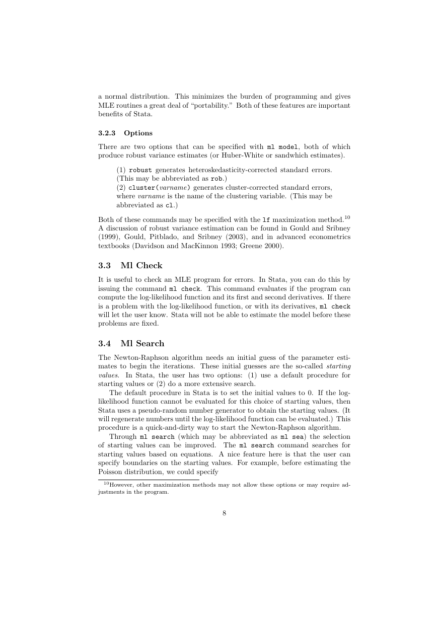
Through ml search (which may be abbreviated as ml sea) the selection
of starting values can be improved. The ml search command searches for
starting values based on equations. A nice feature here is that the user can
specify boundaries on the starting values. For example, before estimating the
Poisson distribution, we could specify
10However, other maximization methods may not allow these options or may require ad-
justments in the program.
8
�


 2023年江西萍乡中考道德与法治真题及答案.doc
 2012年重庆南川中考生物真题及答案.doc
 2013年江西师范大学地理学综合及文艺理论基础考研真题.doc
 2020年四川甘孜小升初语文真题及答案I卷.doc
 2020年注册岩土工程师专业基础考试真题及答案.doc
 2023-2024学年福建省厦门市九年级上学期数学月考试题及答案.doc
 2021-2022学年辽宁省沈阳市大东区九年级上学期语文期末试题及答案.doc
 2022-2023学年北京东城区初三第一学期物理期末试卷及答案.doc
 2018上半年江西教师资格初中地理学科知识与教学能力真题及答案.doc
 2012年河北国家公务员申论考试真题及答案-省级.doc
 2020-2021学年江苏省扬州市江都区邵樊片九年级上学期数学第一次质量检测试题及答案.doc
 2022下半年黑龙江教师资格证中学综合素质真题及答案.doc