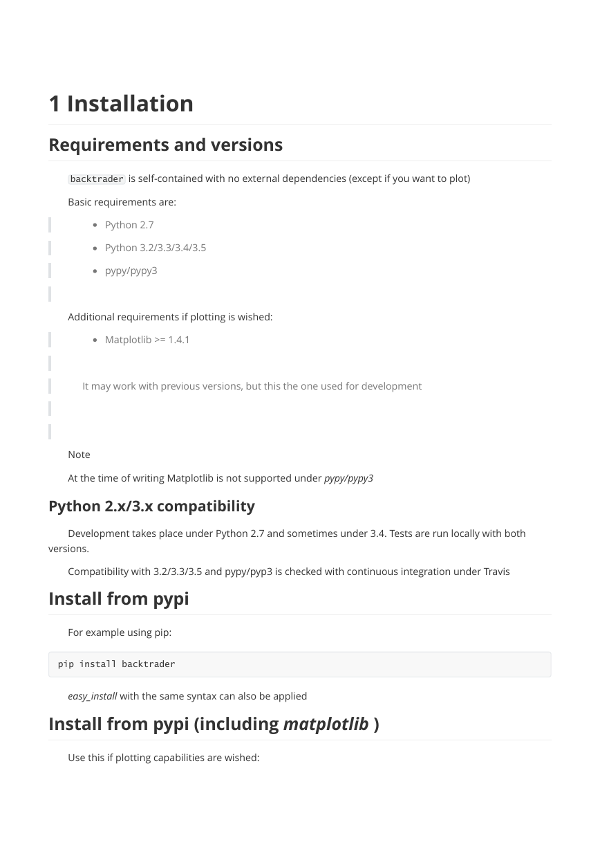
1 Installation
Requirements and versions
Python 2.x/3.x compatibility
Install from pypi
Install from pypi (including matplotlib )
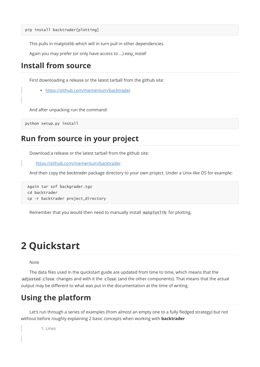
Install from source
Run from source in your project
2 Quickstart
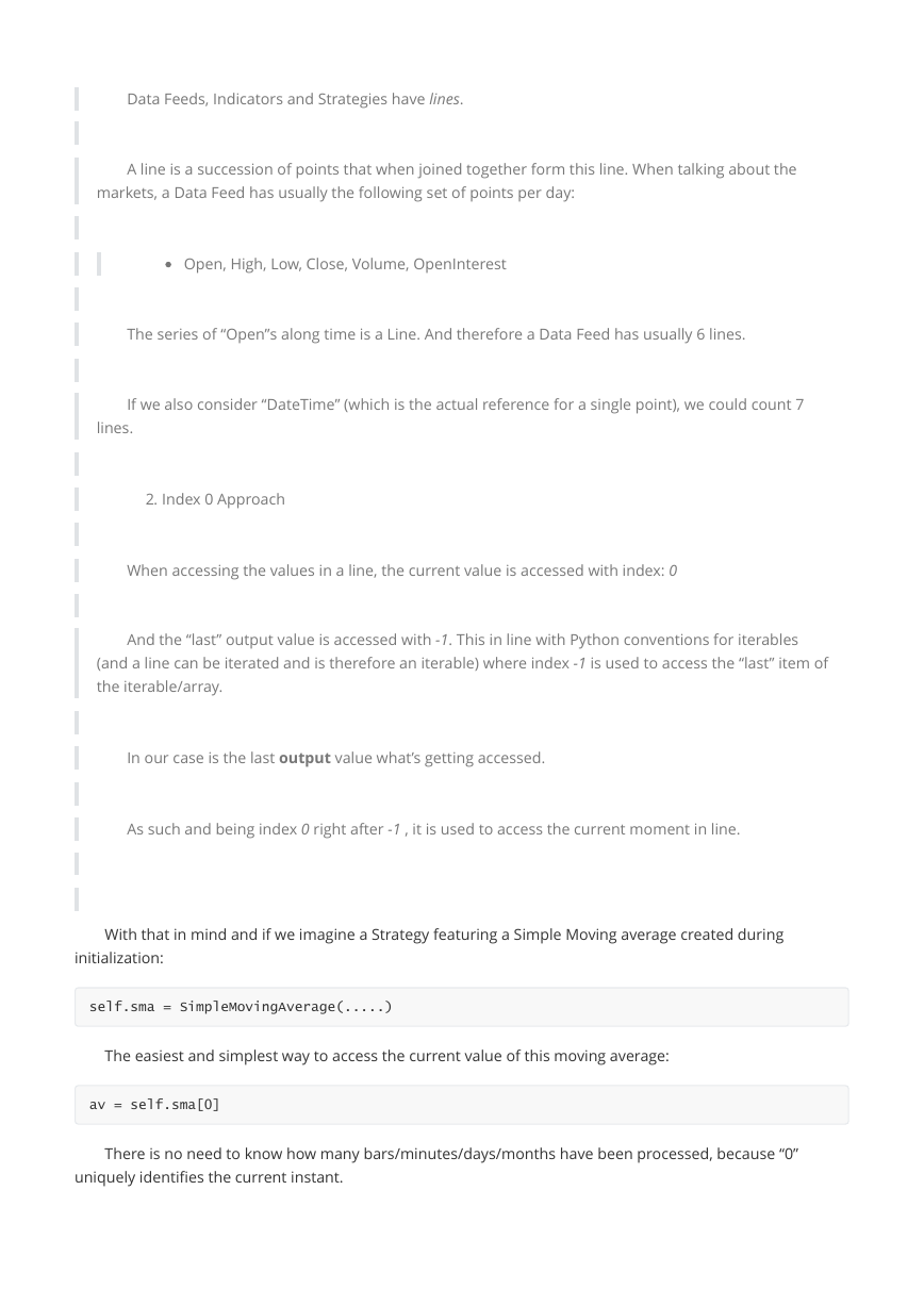
Using the platform
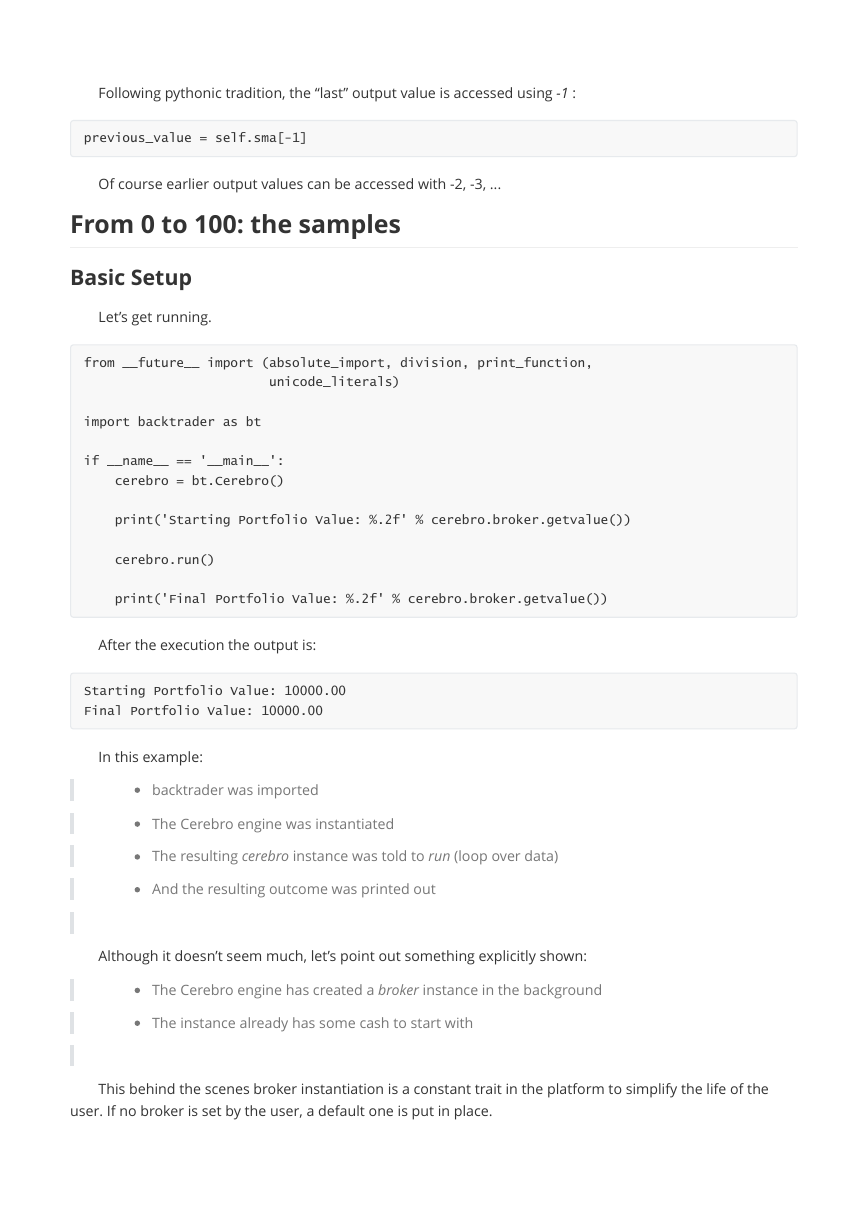
From 0 to 100: the samples
Basic Setup
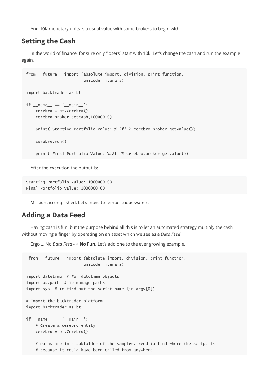
Setting the Cash
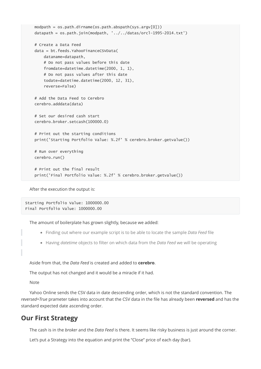
Adding a Data Feed
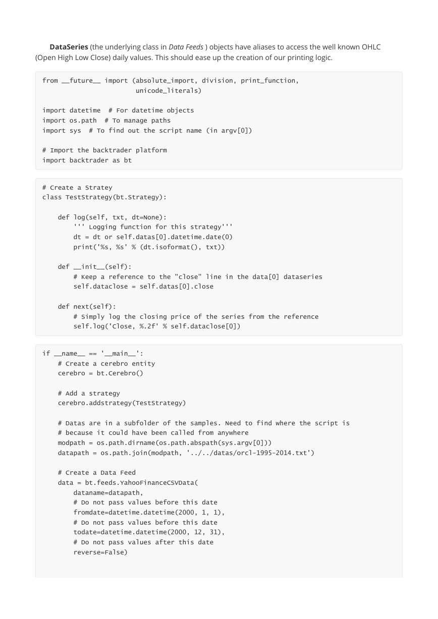
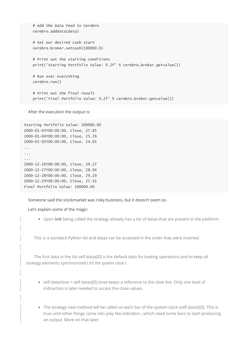
Our First Strategy
Adding some Logic to the Strategy
Do not only buy ... but SELL
The broker says: Show me the money!
Customizing the Strategy: Parameters
Adding an indicator
Visual Inspection: Plotting
Let’s Optimize
Conclusion
3 Platform Concepts
Before Starting
Data Feeds - Passing them around
Shortcuts for Data Feeds
Omitting the Data Feeds
Almost everything is a Data Feed
Parameters
Lines
Lines declaration
Accessing lines in Data Feeds
Lines len
Inheritance of Lines and Params
Params inheritance
Lines Inheritance
Indexing: 0 and -1
Slicing
Getting a slice
Lines: DELAYED indexing
Lines Coupling
Operators, using natural constructs
Stage 1 - Operators Create Objects
Stage 2 - Operators true to nature
Some non-overriden operators/functions
4 Operating the platform
Line Iterators
Extra methods for Indicators
Minimum Period
Up and Running
Data Feeds
A Strategy (derived) class
A Cerebro
5 Exceptions
Hierarchy
Location
Exceptions
StrategySkipError
6 Cerebro
Gathering input
Execute the backtesting
Standard Observers
Returning the results
Giving access to the plotting facilities
Backtesting logic
Reference
7 Cheat On Open
Trying cheat-on-open
Conclusion
Sample usage
Sample source
8 Strategy
How to Buy/Sell/Close
Information Bits:
Member Attributes:
Member Attributes (meant for statistics/observers/analyzers):
Reference: Strategy
9 Sizers - Smart Staking
Using Sizers
From Cerebro
From Strategy
Sizer Development
Practical Sizer Applicability
bt.Sizer Reference
10 Timers
Options
Usage pattern
Adding timers - Via Strategy
Adding timers - Via Cerebro
When are timers called
If cheat=False
If cheat=True
Running with daily bars
Running with 5-minute bars
Additional scenarios
Parameters to add_timer
Sample usage scheduled.py
Sample usage scheduled-min.py
Sample source scheduled.py
Sample source scheduled-min.py
11 Target Orders
The Sample
order_target_size
order_target_value
order_target_percent
Sample Usage
Sample Code
12 Strategy with Signals
Initial FAQ
Signals technicalities
Signals indications
Signals Types
Accumulation and Order Concurrency
The sample
First run: long and short
Second run: long only
Third run: short only
Fourth run: long + longexit
Usage
The code
13 Broker
Reference
14 Slippage
How it works
Configuring slippage
Practical examples
15 Fillers
The fillers signature
Adding a Filler to the broker
The sample
Reference
16 Orders
Order creation
Order notification
Order Status values
Reference: Order and associated classes
17 Order Management and Execution
Order Management
Order Execution Logic
Market
Close
Limit
Stop
StopLimit
Some samples
Execution Type: Market
Execution Type: Close
Execution Type: Limit
Execution Type: Limit with validity
Execution Type: Stop
Execution Type: StopLimit
Test Script Execution
The full code
18 OCO orders
Sample usage
Sample Code
19 StopTrail(Limit)
20 Bracket Orders
Usage Pattern
Single Issuing of a Bracket
Manual Issuing of a Bracket
A sample of it
Some reference
Sample usage
Sample Code
21 Futures and Spot Compensation
Putting it all together
Sample Usage
Sample Code
22 Data Feeds
Data Feeds Common parameters
CSV Data Feeds Common parameters
GenericCSVData
23 CSV Data Feed Development
Caveat Emptor
24 Binary Datafeed Development
Sample binary datafeed
Initialization
Start
Stop
Actual Loading
Other Binary Formats
VChartData Test
VChartData Full Code
25 Extending a Datafeed
6](https://github.com/mementum/backtrader/issues/6)):
6](https://github.com/mementum/backtrader/issues/6)
Plotting that extra P/E line
26 Pandas DataFeed Example
27 Trading Calendar
Trading Calendar Interface
Implementations
PandasMarketCalendar
TradingCalendar
Usage pattern
Global Trading Calendar
Per data-feed
Examples
Daily to Weekly
Minutes to Daily
Extra bonus for the strategy
Sample usage (tcal.py)
Sample usage (tcal-intra.py)
Sample Code (tcal.py)
Sample Code (tcal-intra.py)
28 Data Resampling
29 Data - Multiple Timeframes
Example 1 - Daily and Weekly
Example 2 - Daily and Daily Compression (2 bars to 1)
Example 3 - Strategy with SMA
Invocation 1:
Invocation 2:
Conclusion
30 Data - Replay
Example - Replay Daily to Weekly
Example 2 - Daily to Daily with Compression
Conclusion
31 Rolling over Futures
The RollOver Data Feed
Options for the Roll-Over
Subclassing RollOver
Let’s Roll
Futures concatenation
Futures roll-over with no checks
Changing during the Week
Adding a volume condition
Concluding
Sample Usage
Sample Code
32 Filters
Purpose
Filters at work
Filter Interface
A Sample Filter
Data Pseudo-API for Filters
Another example: Pinkfish Filter
33 Using Indicators
Indicators in action
__init__ vs next
During __init__
During next
The __init__ vs next why
Some notes
Indicator Plotting
Controlling plotting
34 TA-Lib
Requirements
Using ta-lib
Moving Averages and MA_Type
Plotting ta-lib indicators
Examples and comparisons
KAMA (Kaufman Moving Average)
SMA
EMA
Stochastic
RSI
MACD
Bollinger Bands
AROON
Ultimate Oscillator
Trix
ADXR
DEMA
TEMA
PPO
WilliamsR
ROC
Sample Usage
Sample Code
35 Mixing Timeframes in Indicators
Full coupling syntax
Conclusion
Script Code and Usage
36 Indicator Development
Important note: Idempotence
A dummy (but functional) indicator
Manual/Automatic Minimum Period
A full custom indicator
37 Observers and Statistics
Accesing the Observers
Observer Implementation
Adding Observers to the Strategy
Developing Observers
Custom OrderObserver
Saving/Keeping the statistics
38 Benchmarking
Analyzers - Benchmarking
Observers - Benchmarking
Observing TimeReturn
Observing Benchmarking
Observing Benchmarking - Another data
Concluding
The code
39 Analyzers
Nature of analyzers
Location in the ecosystem
Additional Location
Attributes
Returning the analysis
Modus operandi
Analyzer Patterns
A quick example
Forensic Analysis of an Analyzer
Reference
40 PyFolio Overview
Usage
Sample Code
Reference
41 Pyfolio Integration
No PyFolio
A PyFolio run
42 Writer
Reference
43 Commissions: Stocks vs Futures
Agnosticity
Using the broker shortcuts
The meaning of the setcommission parameters
Two examples now: stocks vs futures
Creating permanent Commission schemes
Now a “real” comparison with a SMA Crossover
Commissions for futures
Commissions for stocks
The code
Reference
44 Extending Commissions
Commissions for futures (fixed and with margin)
Commissions for stocks (perc and withoout margin)
Commissions for futures (perc and with margin)
The code for the sample
45 User Defined Commissions
Defining a Commission Scheme
How to apply this to the platform
A practical example
Explaining pseudoexec
CommInfoBase docstring and params
46 Commissions: Credit
Parameters
The formula
Overriding the formula
47 Position
Reference: Position
48 Trade
Reference: Trade
49 Plotting
How to plot
Plotted Elements
Plotting Options
Object-wide plotting options
The meaning of the options
Line specific plotting options
Passing options to a not yet known line
Some plotlines examples
Methods controlling plotting
System-wide plotting options
PlotScheme
Colors in PlotScheme
50 Plotting Date Ranges
Sample Usage
Sample Code
51 Plotting on the same axis
Sample Usage
Sample Code
52 Optimization improvements
Data Feed Management
Results management
Some test runs
Single Core Run
Multiple Core Runs
Both optdata and optreturn active
optreturn deactivated
optdatas deactivated
Both deactivated
Concluding
Sample Usage
53 Automating BackTesting
Applying a User Defined Strategy
Using a built-in Strategy
Using no Strategy
Adding Analyzers
Adding Indicators and Observers
Plotting Control
Usage of the script
54 Saving Memory
Script Code and Usage
55 DateTime Management
Operation with timezones
Datetime Input
Datetime output
56 Live Data Feeds and Live Trading
57 Data Feeds Reference
57 AbstractDataBase
57 BacktraderCSVData
57 CSVDataBase
57 Chainer
57 DataClone
57 DataFiller
57 DataFilter
57 GenericCSVData
57 IBData
57 InfluxDB
57 MT4CSVData
57 OandaData
57 PandasData
57 PandasDirectData
57 Quandl
57 QuandlCSV
57 RollOver
57 SierraChartCSVData
57 VCData
57 VChartCSVData
57 VChartData
57 VChartFile
57 YahooFinanceCSVData
57 YahooFinanceData
57 YahooLegacyCSV
58 Yahoo Data Feed Notes
Using the v7 API/format
Using the legacy API/format
59 Indicator Reference
59 AccelerationDecelerationOscillator
59 Accum
59 AdaptiveMovingAverage
59 AdaptiveMovingAverageEnvelope
59 AdaptiveMovingAverageOscillator
59 AllN
59 AnyN
59 ApplyN
59 AroonDown
59 AroonOscillator
59 AroonUp
59 AroonUpDown
59 AroonUpDownOscillator
59 Average
59 AverageDirectionalMovementIndex
59 AverageDirectionalMovementIndexRating
59 AverageTrueRange
59 AwesomeOscillator
59 BaseApplyN
59 BollingerBands
59 BollingerBandsPct
59 CointN
59 CommodityChannelIndex
59 CrossDown
59 CrossOver
59 CrossUp
59 DV2
59 DemarkPivotPoint
59 DetrendedPriceOscillator
59 DicksonMovingAverage
59 DicksonMovingAverageEnvelope
59 DicksonMovingAverageOscillator
59 DirectionalIndicator
59 DirectionalMovement
59 DirectionalMovementIndex
59 DoubleExponentialMovingAverage
59 DoubleExponentialMovingAverageEnvelope
59 DoubleExponentialMovingAverageOscillator
59 DownDay
59 DownDayBool
59 DownMove
59 Envelope
59 ExponentialMovingAverage
59 ExponentialMovingAverageEnvelope
59 ExponentialMovingAverageOscillator
59 ExponentialSmoothing
59 ExponentialSmoothingDynamic
59 FibonacciPivotPoint
59 FindFirstIndex
59 FindFirstIndexHighest
59 FindFirstIndexLowest
59 FindLastIndex
59 FindLastIndexHighest
59 FindLastIndexLowest
59 Fractal
59 HeikinAshi
59 Highest
59 HullMovingAverage
59 HullMovingAverageEnvelope
59 HullMovingAverageOscillator
59 HurstExponent
59 Ichimoku
59 KnowSureThing
59 LaguerreFilter
59 LaguerreRSI
59 LinePlotterIndicator
59 Lowest
59 MACD
59 MACDHisto
59 MeanDeviation
59 MinusDirectionalIndicator
59 Momentum
59 MomentumOscillator
59 MovingAverageBase
59 MovingAverageSimple
59 MovingAverageSimpleEnvelope
59 MovingAverageSimpleOscillator
59 OLS_BetaN
59 OLS_Slope_InterceptN
59 OLS_TransformationN
59 OperationN
59 Oscillator
59 OscillatorMixIn
59 ParabolicSAR
59 PercentChange
59 PercentRank
59 PercentagePriceOscillator
59 PercentagePriceOscillatorShort
59 PeriodN
59 PivotPoint
59 PlusDirectionalIndicator
59 PrettyGoodOscillator
59 PriceOscillator
59 RSI_EMA
59 RSI_SMA
59 RSI_Safe
59 RateOfChange
59 RateOfChange100
59 ReduceN
59 RelativeMomentumIndex
59 RelativeStrengthIndex
59 Signal
59 SmoothedMovingAverage
59 SmoothedMovingAverageEnvelope
59 SmoothedMovingAverageOscillator
59 StandardDeviation
59 Stochastic
59 StochasticFast
59 StochasticFull
59 SumN
59 TripleExponentialMovingAverage
59 TripleExponentialMovingAverageEnvelope
59 TripleExponentialMovingAverageOscillator
59 Trix
59 TrixSignal
59 TrueHigh
59 TrueLow
59 TrueRange
59 TrueStrengthIndicator
59 UltimateOscillator
59 Buying Pressure = Close - TrueLow BP = Close - Minimum(Low or Prior Close)
59 TrueRange = TrueHigh - TrueLow TR = Maximum(High or Prior Close) -
59 UpDay
59 UpDayBool
59 UpMove
59 Vortex
59 WeightedAverage
59 WeightedMovingAverage
59 WeightedMovingAverageEnvelope
59 WeightedMovingAverageOscillator
59 WilliamsAD
59 WilliamsR
59 ZeroLagExponentialMovingAverage
59 ZeroLagExponentialMovingAverageEnvelope
59 ZeroLagExponentialMovingAverageOscillator
59 ZeroLagIndicator
59 ZeroLagIndicatorEnvelope
59 ZeroLagIndicatorOscillator
59 haDelta
60 TA-Lib Indicator Reference
TA-Lib Indicator Reference
61 Strategies Reference
61 MA_CrossOver
61 SignalStrategy
62 Analyzers Reference
AnnualReturn
Calmar
DrawDown
TimeDrawDown
GrossLeverage
PositionsValue
PyFolio
LogReturnsRolling
PeriodStats
Returns
SharpeRatio
SharpeRatio_A
SQN
TimeReturn
TradeAnalyzer
Transactions
VWR
63 Observers Reference
Benchmark
Broker
Broker - Cash
Broker - Value
BuySell
DrawDown
TimeReturn
Trades
LogReturns
LogReturns2
FundValue
FundShares
64 Sizers Reference
FixedSize
FixedReverser
PercentSizer
AllInSizer
65 Filters Reference
SessionFilter
SessionFilterSimple
SessionFilller
CalendarDays
BarReplayer_Open
DaySplitter_Close
HeikinAshi
Renko


 2023年江西萍乡中考道德与法治真题及答案.doc
 2012年重庆南川中考生物真题及答案.doc
 2013年江西师范大学地理学综合及文艺理论基础考研真题.doc
 2020年四川甘孜小升初语文真题及答案I卷.doc
 2020年注册岩土工程师专业基础考试真题及答案.doc
 2023-2024学年福建省厦门市九年级上学期数学月考试题及答案.doc
 2021-2022学年辽宁省沈阳市大东区九年级上学期语文期末试题及答案.doc
 2022-2023学年北京东城区初三第一学期物理期末试卷及答案.doc
 2018上半年江西教师资格初中地理学科知识与教学能力真题及答案.doc
 2012年河北国家公务员申论考试真题及答案-省级.doc
 2020-2021学年江苏省扬州市江都区邵樊片九年级上学期数学第一次质量检测试题及答案.doc
 2022下半年黑龙江教师资格证中学综合素质真题及答案.doc