稀疏表示SAR成像.pdf

发布时间：2022-06-18 发布人：admin 分类：说明书资料大小：0.67M 资料格式：pdf 举报版权申诉

7d405971-1d0a-4ad5-86e6-fb51a99a09b3.pdf-第1页.png

第1页 / 共13页

7d405971-1d0a-4ad5-86e6-fb51a99a09b3.pdf-第2页.png

第2页 / 共13页

7d405971-1d0a-4ad5-86e6-fb51a99a09b3.pdf-第3页.png

第3页 / 共13页

7d405971-1d0a-4ad5-86e6-fb51a99a09b3.pdf-第4页.png

第4页 / 共13页

7d405971-1d0a-4ad5-86e6-fb51a99a09b3.pdf-第5页.png

第5页 / 共13页

7d405971-1d0a-4ad5-86e6-fb51a99a09b3.pdf-第6页.png

第6页 / 共13页

7d405971-1d0a-4ad5-86e6-fb51a99a09b3.pdf-第7页.png

第7页 / 共13页

7d405971-1d0a-4ad5-86e6-fb51a99a09b3.pdf-第8页.png

第8页 / 共13页

toc

A Sparse Signal Reconstruction Perspective for Source Localizati

Dmitry Malioutov, Student Member, IEEE, Müjdat Çetin, Member, IE

I. I NTRODUCTION

II. S PARSE S IGNAL R EPRESENTATION

III. S OURCE L OCALIZATION F RAMEWORK

A. Source Localization Problem

B. Overcomplete Representation for a Single Time Sample

Fig.€1. Single sample source localization with $\ell_1$ . Spatia

IV. S OURCE L OCALIZATION W ITH M ULTIPLE T IME S AMPLES AND $\e

A. Treating Each Time Index Separately

B. Joint-Time Inverse Problem

C. $\ell_1$ -SVD

Fig.€2. Block diagram of steps for $\ell_1$ -SVD.

V. SOC R EPRESENTATION OF THE $\ell_1$ -SVD P ROBLEM

VI. M ULTIRESOLUTION G RID R EFINEMENT

Fig.€3. Illustration of grid refinement.

VII. R EGULARIZATION P ARAMETER S ELECTION

VIII. E XPERIMENTAL R ESULTS

Fig.€4. (a) and (b). Spatial spectra for beamforming, Capon's me

A. Spectra for $\ell_1$ -SVD

Fig. 5. Spectra for correlated sources. ${\hbox{SNR}} = 20$ dB.

Fig. 6. Comparison with beamspace technique of [ 14 ] . ${\hbox{

Fig.€7. Resolving $M-1$ sources: $M=8$ sensors, seven sources, $

Fig.€8. Sensitivity of MUSIC to the assumed number of sources. T

Fig.€9. Sensitivity of $\ell_1$ -SVD to the assumed number of so

B. Regularization Parameter Choice

Fig.€10. Regularization parameter choice: Discrepancy principle

Fig.€11. Regularization parameter choice for moderate noise: Rat

C. Bias and Variance

Fig.€12. Bias of $\ell_1$ -SVD in localizing two sources as a fu

Fig.€13. CRB for zero mean uncorrelated sources. Comparison with

Fig.€14. Plots of variances of DOA estimates versus SNR, as well

D. Wideband Source Localization

Fig.€15. (a) and (b). Wideband example: Three chirps. DOAs: 70 $

Fig.€16. Joint coherent processing of multiple harmonics with sp

IX. C ONCLUSION

F ORMULATING $\ell_1$ -SVD AS A SOC O PTIMIZATION P ROBLEM

H. Krim and M. Viberg, Two decades of array signal processing re

D. H. Johnson and D. E. Dudgeon, Array Signal Processing Concept

R. O. Schmidt, A Signal Subspace Approach to Multiple Emitter Lo

J. Capon, High resolution frequency-wavenumber spectrum analysis

P. Charbonnier, L. Blanc-Féraud, G. Aubert, and M. Barlaud, Dete

S. Sardy, P. Tseng, and A. Bruce, Robust wavelet denoising, IEEE

P. S. Bradley, O. L. Mangasarian, and W. N. Street, Feature sele

M. Çetin and W. C. Karl, Feature-enhanced synthetic aperture rad

R. Tibshirani, Regression shrinkage and selection via the LASSO,

M. D. Sacchi, T. J. Ulrych, and C. J. Walker, Interpolation and

B. D. Jeffs, Sparse inverse solution methods for signal and imag

I. F. Gorodnitsky and B. D. Rao, Sparse signal reconstruction fr

J. J. Fuchs, Linear programming in spectral estimation. Applicat

B. D. Rao and K. Kreutz-Delgado, An affine scaling methodology f

S. S. Chen, D. L. Donoho, and M. A. Saunders, Atomic decompositi

S. Mallat and Z. Zhang, Matching pursuits with time-frequency di

D. M. Malioutov, M. Cetin, and A. S. Willsky, Optimal sparse rep

A. J. Miller, Subset Selection in Regression . London, U.K.: Cha

D. M. Malioutov . (2003, Jul.) A Sparse Signal Reconstruction Pe

D. L. Donoho and M. Elad, Maximal sparsity representation via l1

R. Gribonval and M. Nielsen, Sparse representation in unions of

J. J. Fuchs, More on sparse representations in arbitrary bases,

R. Gribonval and M. Nielsen, Highly sparse representations from

J. A. Tropp, Greed is Good: Algorithmic Results for Sparse Appro

D. L. Donoho, M. Elad, and V. Temlyakov, Stable recovery of spar

J. A. Tropp, Just relax: Convex programming methods for subset s

D. L. Donoho, Superresolution via sparsity constraints, SIAM J.

J. J. Fuchs, Detection and estimation of superimposed signals, i

B. D. Rao and K. Kreutz-Delgado, Basis selection in the presense

M. Lobo, L. Vandenberghe, S. Boyd, and H. Lebret, Applications o

A. Nemirovski and A. Ben Tal, Lectures on Modern Convex Optimiza

J. S. Sturm . (2001) Using SeDuMi 1.02, a Matlab Toolbox for Opt

V. A. Morozov, On the solution of functional equations by the me

P. C. Hansen, Analysis of discrete ill-posed problems by means o

B. D. Rao, K. Engan, S. F. Cotter, J. Palmer, and K. Kreutz-Delg

S. Sivanand, J. F. Yang, and M. Kaveh, Time-domain coherent sign

3010 IEEE TRANSACTIONS ON SIGNAL PROCESSING, VOL. 53, NO. 8, AUGUST 2005 A Sparse Signal Reconstruction Perspective for Source Localization With Sensor Arrays Dmitry Malioutov, Student Member, IEEE, Müjdat Çetin, Member, IEEE, and Alan S. Willsky, Fellow, IEEE Abstract—We present a source localization method based on a sparse representation of sensor measurements with an overcom- plete basis composed of samples from the array manifold. We enforce sparsity by imposing penalties based on the 1-norm. A number of recent theoretical results on sparsifying properties of 1 penalties justify this choice. Explicitly enforcing the sparsity of the representation is motivated by a desire to obtain a sharp estimate of the spatial spectrum that exhibits super-resolution. We propose to use the singular value decomposition (SVD) of the data matrix to summarize multiple time or frequency samples. Our formulation leads to an optimization problem, which we solve efﬁciently in a second-order cone (SOC) programming framework by an interior point implementation. We propose a grid reﬁnement method to mitigate the effects of limiting estimates to a grid of spatial locations and introduce an automatic selection criterion for the regularization parameter involved in our approach. We demonstrate the effectiveness of the method on simulated data by plots of spatial spectra and by comparing the estimator variance to the Cramér–Rao bound (CRB). We observe that our approach has a number of advantages over other source localization techniques, including increased resolution, improved robustness to noise, limitations in data quantity, and correlation of the sources, as well as not requiring an accurate initialization. Index Terms—Direction-of-arrival estimation, overcomplete representation, sensor array processing, source localization, sparse representation, superresolution. I. INTRODUCTION S OURCE localization using sensor arrays [1], [2] has been an active research area, playing a fundamental role in many applications involving electromagnetic, acoustic, and seismic sensing. An important goal for source localization methods is to be able to locate closely spaced sources in presence of con- siderable noise. Many advanced techniques for the localization of point sources achieve superresolution by exploiting the pres- ence of a small number of sources. For example, the key com- ponent of the MUSIC method [3] is the assumption of a low-di- mensional signal subspace. We follow a different approach for exploiting such a structure: We pose source localization as an overcomplete basis representation problem, where we impose a penalty on the lack of sparsity of the spatial spectrum. Our approach is distinctly different from the existing source localization methods, although it shares some of their ingre- dients. The most well-known existing nonparametric methods Manuscript received April 26, 2004; revised November 5, 2004. This work was supported by the Army Research Ofﬁce under Grant DAAD19-00-1-0466 and the Air Force Ofﬁce of Scientiﬁc Research under Grant F49620-00-1-0362. The associate editor coordinating the review of this manuscript and apporovng it for publication was Dr. Jean Pierre Delmas. The authors are with the Department of Electrical Engineering and Computer Science, Massachusetts Institute of Technology, Cambridge, MA 02139 USA. Digital Object Identiﬁer 10.1109/TSP.2005.850882 include beamforming [2], Capon’s method [4], and subspace- based methods such as MUSIC [3]. Some additional methods (Root-MUSIC and ESPRIT) [1] require the assumption that the array of sensors is linear. Beamforming spectrum suffers from the Rayleigh resolution limit, which is independent of the SNR. MUSIC and Capon’s method are able to resolve sources within a Rayleigh cell (i.e., achieve super-resolution), provided that the SNR is moderately high, the sources are not strongly correlated, and the number of snapshots is sufﬁcient. A family of parametric methods based on the maximum likelihood paradigm, including deterministic maximum likelihood (DML) and stochastic max- imum likelihood (SML) [1], enjoy excellent statistical proper- ties, but an accurate initialization is required to converge to a global minimum. By turning to the sparse signal representation framework, we are able to achieve super-resolution without the need for a good initialization, without a large number of time samples, and with lower sensitivity to SNR and to correlation of the sources. -norm penalty with The topic of sparse signal representation has evolved very rapidly in the last decade, ﬁnding application in a variety of problems, including image reconstruction and restoration [5], wavelet denoising [6], feature selection in machine learning [7], radar imaging [8], and penalized regression [9]. There has also been some emerging investigation of these ideas in the context of spectrum estimation and array processing [10]–[14]. Sacchi et al. [10] use a Cauchy-prior to enforce sparsity in spectrum estimation and solve the resulting optimization problem by iter- to ative methods. Jeffs [11] uses an enforce sparsity for a number of applications, including sparse antenna array design. Gorodnitsky et al. [12] apply a recur- sive weighted minimum-norm algorithm called focal underde- termined system solver (FOCUSS) to achieve sparsity in the problem of source localization. It was later shown [15] that penalties with the algorithm is related to the optimization of . The work of Fuchs [13], [14] is concerned with source localization in the beamspace domain, under the assumption that the sources are uncorrelated, and that a large number of time samples is available. The method attempts to represent the vector of beamformer outputs to unknown sources as a sparse linear combination of vectors from a basis of beamformer out- puts to isolated unit power sources. The method uses the penalty for sparsity and the penalty for noise. Prior research has established sparse signal representation as a valuable tool for signal processing, but its application to source localization has been developed only for very limited scenarios. We start with the ideas of enforcing sparsity by penalties and extend them to a general framework that is applicable to a wide variety of practical source localization problems. In its most basic form, the problem of sparse signal repre- sentation in overcomplete bases asks to ﬁnd the sparsest signal 1053-587X/$20.00 © 2005 IEEE

MALIOUTOV et al.: SPARSE SIGNAL RECONSTRUCTION PERSPECTIVE FOR SOURCE LOCALIZATION WITH SENSOR ARRAYS 3011 , where to satisfy basis, i.e., is an overcomplete . Without the sparsity prior on , the problem is ill-posed and has inﬁnitely many solutions. Addi- should be sufﬁciently sparse allows tional information that one to get rid of the ill-posedness. Solving problems involving sparsity typically requires combinatorial optimization, which is intractable even for modest data sizes; therefore, a number of re- laxations have been considered [16]–[19]. We give a brief syn- opsis of relevant ideas in sparse signal representation in Sec- tion II. The application of this methodology to practical array processing problems requires being able to handle additive noise, using multiple time or frequency samples from possibly strongly correlated sources in a sensible fashion, and allowing the data to be complex: (1) The goal of this paper is to explore how to utilize the sparse signal representation methodology for practical narrowband and wideband source localization using sensor arrays. The main contributions of our paper include a new adaptation of sparse signal representation to source localization through the development of an approach based on the singular value decomposition (SVD) to combine multiple samples and the use of second-order cone programming for optimization of the resulting objective function. The key ingredients of the proposed method is the use of SVD for data reduction and the formulation of a joint multiple-sample sparse representation problem in the signal subspace domain. In the body of the -SVD. In addition, we paper, we refer to the method as introduce the idea of adaptive grid reﬁnement to combat the effects of a bias introduced by a limitation of the estimates to a grid. Finally, we discuss a method for the automatic selection of the regularization parameter involved in our approach, which -SVD objective. balances data-ﬁdelity with sparsity in the In our experiments, the proposed approach exhibits a number of advantages over other source localization techniques, which include increased resolution, and improved robustness to noise, to limited number of snapshots, and to correlation of the sources. In addition, due to the convexity of all the optimization tasks involved in the approach, it does not require an accurate initialization. Another advantage of the approach is its ﬂexi- bility, since few assumptions are made in the formulation, e.g., the array does not have to be linear, and the sources may be strongly correlated. Similarly, extensions to many scenarios, such as distributed sources and non-Gaussian noise, can be readily made. In the paper, we mostly focus on the narrow- band farﬁeld problem with arbitrary array geometry; we also describe the wideband scenario brieﬂy in Section VIII-D. A more extensive discussion can be found in [20], where we also consider beamspace versions, cover wideband and nearﬁeld processing in more detail, and propose an approach for simul- taneous self-calibration and source localization in the presence of model errors. We start with a brief introduction to the problem of sparse signal representation in Section II. In Section III, we describe the source localization problem and represent a single sample problem directly in the sparse signal representation framework. In Section IV, we extend the approach to handle multiple sam- ples. This is done in several steps, leading to the -SVD tech- nique. In Section V, we describe how to ﬁnd numerical solutions via a second-order cone programming (SOC) framework. We describe how to eliminate the effects of the grid in Section VI and propose how to automatically choose a regularization pa- rameter involved in our approach in Section VII. Finally, in Sec- tion VIII, the advantages and disadvantages of the framework are explored using simulated experiments, and conclusions are made in Section IX. II. SPARSE SIGNAL REPRESENTATION , given , with . The matrix , which we also call the The simplest version of the sparse representation problem , without noise is to ﬁnd a sparse which are related by is known. The assumption of sparsity of problem is ill-posed without it ( An ideal measure of sparsity is the count of nonzero entries which is denoted by Hence, mathematically, we must look for arg min is crucial since the has a nontrivial null-space). , -norm.1 such that . This is, however, a difﬁcult combinatorial optimiza- tion problem and is intractable for even moderately sized prob- lems. Many approximations have been devised over the years, including greedy approximations (matching pursuit, stepwise regression, and their variants [17], [19]), as well as re- laxations, where , for , [20]. For the latter two, it has been shown recently that if , then these approxi- mations in fact lead to exact solutions (see [18], [20]–[24] for precise deﬁnitions of these notions).2 In addition, [26] and [27] showed that with sufﬁcient sparsity and a favorable structure of the overcomplete basis, sparse representations are stable in the presence of noise. These results are practically very signiﬁcant is a convex since the optimization problem, and the global optimum can be found for real-valued data by linear programming.3 As these equivalence results are not specialized to the source localization problem but are derived for general overcomplete bases, the bounds that they provide are loose. A result that does take the structure of the basis into account is developed in [28]. is “sparse enough” with respect to is replaced by , [16], and relaxation subject to and In practice, a noiseless measurement model is rarely appro- priate; therefore, noise must be introduced. A sparse represen- tation problem with additive Gaussian noise takes the following form: (2) To extend choice of an optimization criterion is -penalization to the noisy case, an appropriate subject to is a parameter specifying how , where 1The symbols kxk and kxk are both used in the literature to represent the count of nonzero elements. We use the latter symbol since in the limit as p ! 0 ; kxk approaches the count of nonzero elements, but, if x 6= 0 kxk ! 1. 2Recent studies of greedy methods, which have lower complexity than ` and ` -based methods, have also yielded theoretical results of a similar ﬂavor [25], [26]. 3In addition, for the ` problem, local minima can be readily found by con- tinuous optimization methods, as described in [20].

3012 IEEE TRANSACTIONS ON SIGNAL PROCESSING, VOL. 53, NO. 8, AUGUST 2005 much noise we wish to allow. An unconstrained form of this objective is (3) This objective function has been used in a number of sparse signal representation works ([16], [29] for real-valued data and -term forces the residual [30] for complex-valued data). The -term enforces sparsity of the to be small, whereas the representation. The parameter controls the tradeoff between the sparsity of the spectrum and the residual norm. We use these ideas in Sections III and IV for source localization. The optimization criterion is again a convex optimization problem and can be readily handled by quadratic programming for real data. We propose the use of SOC programming for the complex data case. We describe SOC programming in Section V. . However, for penalty instead of The class of methods called FOCUSS [12] is another par- adigm for solving sparse signal representation problems with , a more general the cost function is nonconvex, and the convergence to global minima is not guaranteed. The discussion in [15] in Section VI indicates that the best results are obtained for close to 1, whereas the convergence is also slowest for . The cost per iteration for FOCUSS methods is similar to that of an interior point solver for SOC since both solve a modiﬁed Newton’s method step of similar dimensions. However, the number of iterations of SOC is better behaved (in fact, there are bounds on the worst-case number of iterations for SOC [31]) than for FOCUSS with . In our previous work [20], we have also observed slow convergence of iterative algorithms for . By using an SOC minimization when applied with formulation that is tailored to the convex case, we are able to achieve fast convergence and guarantee global optimality of the solution. III. SOURCE LOCALIZATION FRAMEWORK A. Source Localization Problem The goal of sensor array source localization is to ﬁnd the lo- cations of sources of waveﬁelds that impinge on an array con- sisting of a number of sensors. The available information is the geometry of the array, the parameters of the medium where waveﬁelds propagate, and the measurements on the sensors. For purposes of exposition, we ﬁrst focus on the narrow- band scenario and delay the presentation of wideband source localization until Section VIII-D. Consider narrowband sig- nals om- nidirectional sensors, after being corrupted by additive noise . Let . After demodulation, the basic narrowband observation model can be expressed as [1], [2] , resulting in sensor outputs , arriving at an array of and similarly deﬁne and (4) The matrix is the so-called array manifold matrix, whose th element contains the delay and gain information from th sensor. The columns ) to the the th source (at location of , for , are called steering vec- tors. The number of sources is unknown. To simplify the ex- position, we only discuss the farﬁeld scenario and conﬁne the array to a plane, although neither of these assumptions is re- quired for our approach. With farﬁeld sources in the same plane as the array, the unknown locations of the sources are parame- terized by angles (directions of arrival) with respect to the array and the axis mapping , the goal is to ﬁnd the unknown locations of the sources . Given the knowledge of , as well as their number for all . B. Overcomplete Representation for a Single Time Sample Now, we start to formulate the source localization problem as a sparse representation problem. The single-sample formulation in this section parallels the one in [12], where it was presented as one of applications of FOCUSS algorithm. In addition, the work in [13] and [14] is based on a similar philosophy of trans- forming a parameter estimation problem into sparse spectrum estimation, which we discuss later in this section. We consider the single time sample case in this section, with in (4). The problem as it appears in (4) is a nonlinear pa- rameter estimation problem, where the goal is to ﬁnd . Matrix , so it is not depends on the unknown source locations known. To cast this problem as a sparse representation problem, we introduce an overcomplete representation in terms of all possible source locations. Let be a sam- pling grid of all source locations of interest. The number of potential source locations will typically be much greater or even the number of sensors than the number of sources . We construct a matrix composed of steering vectors cor- responding to each potential source location as its columns: is known . In this framework and does not depend on the actual source locations . We represent the signal ﬁeld by an vector , where the th element comes from for some sample, the problem is reduced to is nonzero and equal to if source and zero otherwise. For a single time (5) In effect, this overcomplete representation allows us to for the exchange the problem of parameter estimation of problem of sparse spectrum estimation of . As in numerous nonparametric source localization techniques, the approach forms an estimate of the signal energy as a function of hypoth- esized source location, which ideally contains dominant peaks at the true source locations. The central assumption is that the sources can be viewed as point sources, and their number is small. With this assumption, the underlying spatial spectrum is sparse (i.e., has only a few nonzero elements), and we can solve this inverse problem via regularizing it to favor sparse signal ﬁelds using the methodology, as described in Sec- tion II. The appropriate objective function for the problem is We discuss how is chosen in Section VII, but for now, we as- sume that a good choice can be made. The data for the model (6)

MALIOUTOV et al.: SPARSE SIGNAL RECONSTRUCTION PERSPECTIVE FOR SOURCE LOCALIZATION WITH SENSOR ARRAYS 3013 a penalty that enforces the same sparsity proﬁle over all these vectors, thus imposing temporal coherence. The resulting for- mulation is considerably more general than the one in [14]. IV. SOURCE LOCALIZATION WITH MULTIPLE TIME SAMPLES AND -SVD Single snapshot processing may have its own applications, but source localization with multiple snapshots4 from poten- tially correlated sources is of greater practical importance. When we bring time into the picture, the overcomplete repre- sentation is easily extended. The general narrowband source localization problem with multiple snapshots reformulated using an overcomplete representation has the following form: (7) However, the numerical solution of this problem is a bit more involved than that of the single sample case. In Section IV-A, we describe a simple and computationally efﬁcient method that, however, does not use the snapshots in synergy. In Section IV-B, we propose a coherent method that does use the snapshots in synergy but is more demanding computationally, and in Sec- tion IV-C, we develop an SVD-based approach that dramati- cally reduces the computational complexity while still using the snapshots coherently. A. Treating Each Time Index Separately The ﬁrst thought that comes to mind when we switch from one time sample to several time samples is to solve each problem indexed by separately. In that case, we would have a set of solutions . If the sources are moving fast, then the evolution of is of interest, and the approach is suitable for displaying it. However, when the sources are stationary over several time samples, then it is preferable to combine the independent esti- mates to get one representative estimate of source locations from them, for example, by averaging or by clustering. This is noncoherent averaging, and its main attraction is its simplicity. However, by turning to fully coherent combined processing, as described in the following sections, we expect to achieve greater accuracy and robustness to noise. B. Joint-Time Inverse Problem Now, we consider a simple approach that uses different time samples in synergy. Let and similarly. Then, (7) becomes , and deﬁne (8) There is an important difference of (8) from (5): Matrix is parameterized temporally and spatially, but sparsity only has to be enforced in space since the signal in not generally sparse in time. To accommodate this issue, we impose a different prior: one that requires sparsity in the spatial dimension but does not require sparsity in time. This can be done5 by ﬁrst computing the , -norm of all time-samples of a particular spatial index of 4While here we focus on multiple time snapshots, we will also use the same ideas applied to frequency snapshots for wideband source localization in Sec- tion VIII. 5It came to our attention that a similar idea has been used in [30] for basis selection. 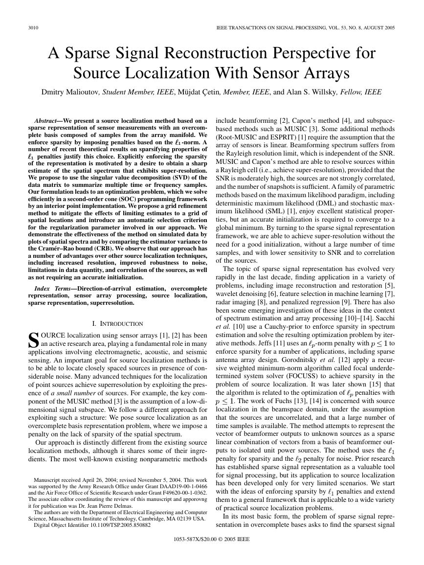Fig. 1. Single sample source localization with ` . Spatial spectra of two sources with DOAs of 60 and 70 (SNR = 20 dB). is complex-valued; hence, neither linear nor quadratic program- ming can be used for numerical optimization. Instead, we adopt an SOC programming framework, which we introduce in Sec- tion V. Once is found, the estimates of the source locations correspond to the locations of the peaks in . We illustrate the approach for source localization with a single time sample in Fig. 1. We consider a uniform linear array of sensors separated by half a wavelength of the actual narrowband source signals. We consider two narrowband signals in the far-ﬁeld impinging on this array from directiions of arrival (DOAs) 60 and 70 , which are closer together than the Rayleigh limit. The SNR is 20 dB. The regularization parameter in this example is chosen by subjective assess- ment. We do not consider other source localization methods such as MUSIC or Capon’s method in this simulation because they rely on estimating the covariance matrix of the sensor measurements, but in the simulation only, one time sample is present. Using beamforming, the two peaks of the spectrum are merged, but using the sparse regularization approach, they are well resolved, and the sidelobes are suppressed almost to zero. Apart from a small asymptotic bias, which we discuss in Section VIII, the spectrum estimate is an example of what super-resolution source localization methods aim to achieve. The work of Fuchs [13], [14] is based on a similar philosophy of transforming a parameter estimation problem into a sparse spectrum estimation problem. A basis composed of beamformer outputs to isolated unit power sources from a large number of directions is created ﬁrst. The method then attempts to represent the vector of beamformer outputs corresponding to the unknown sources as a sparse linear combination of vectors from the basis, using penalties for noise, and opti- mization by quadratic programming. However, this beamspace domain formulation combines the multiple snapshots in a way that requires assumptions that the sources are uncorrelated and that a large number of samples is available. In contrast, the sensor-domain method that we propose in Section IV-C treats the multiple time samples in a very different way: We sum- marize multiple snapshots by using the SVD and solve a joint optimization problem over several singular vectors, imposing penalties for sparsity,

3014 i.e., -norm of , and penalizing the . The cost function becomes (9) The Frobenius norm is deﬁned as . The optimization is performed over vec is a function of . The time samples are combined using the 2-norm, which has no sparsifying effects. The spatial samples -norm, which does enforce sparsity. are combined using the Compared to the independent sample by sample processing from Section IV-A, the different time-indices of reinforce each other, since the penalty is higher if the supports of for different do not line up exactly. Once an estimate of computed using the new cost function, the peaks of the source locations. is provide The main drawback of this technique is its computational cost. The size of the inverse problem increases linearly with , and the computational effort required to solve it increases is large, this approach is superlinearly with not viable for the solution of the real-time source localization problem. We propose a solution to this problem next. . Thus, when C. -SVD In this section, we present a tractable approach to use a large number of time samples coherently, thus extending the use of sparse signal representation ideas for practical source localiza- tion problems. To reduce both the computational complexity and the sensitivity to noise, we use the SVD of the data matrix . The idea is to decompose the data matrix into the signal and noise subspaces, keep the signal subspace, and mold the problem with reduced dimensions into the multiple-sample sparse spectrum estimation problem in the form of Section IV-B. Note that we keep the signal subspace and not the noise subspace, which gets used in MUSIC, Pisarenko, and the minimum norm subspace methods. Without noise on the sensors, the set of vectors vectors instead of -dimensional subspace, where would lie in a is the number of sources.6 We would only need to keep a basis for the subspace ( ) to estimate what sparse combinations form it. With additive noise, we decompose the of columns of data matrix into its signal and noise subspaces and keep a basis for the signal subspace. Mathematically, this translates into the following representation. Take the SVD7 dimensional matrix Keep a reduced tains most of the signal power where is a and , to obtain . Here, matrix of zeros. In addition, let is a identity matrix, and (10) , which con- , , (11) 6If T < K, or if the sources are coherent, we use the number of signal subspace singular values instead of K. 7This is closely related to the eigen-decomposition of the correla- tion matrix of the data: R = 1=T YY . Its eigen-decomposition is R = 1=T ULV VL U = 1=T UL U . IEEE TRANSACTIONS ON SIGNAL PROCESSING, VOL. 53, NO. 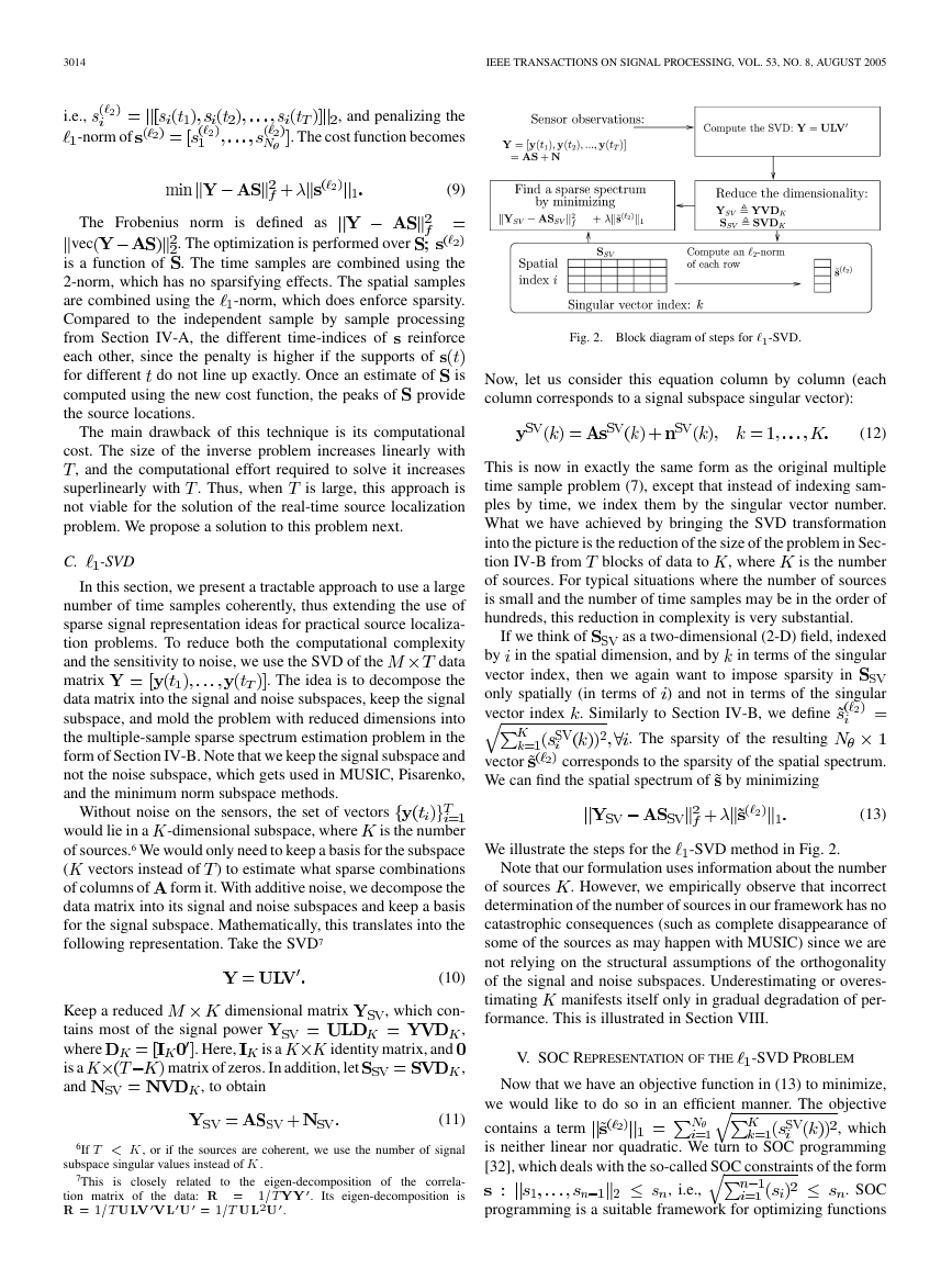8, AUGUST 2005 Fig. 2. Block diagram of steps for ` -SVD. Now, let us consider this equation column by column (each column corresponds to a signal subspace singular vector): (12) This is now in exactly the same form as the original multiple time sample problem (7), except that instead of indexing sam- ples by time, we index them by the singular vector number. What we have achieved by bringing the SVD transformation into the picture is the reduction of the size of the problem in Sec- tion IV-B from blocks of data to is the number of sources. For typical situations where the number of sources is small and the number of time samples may be in the order of hundreds, this reduction in complexity is very substantial. , where If we think of as a two-dimensional (2-D) ﬁeld, indexed in terms of the singular by in the spatial dimension, and by vector index, then we again want to impose sparsity in only spatially (in terms of vector index . Similarly to Section IV-B, we deﬁne . The sparsity of the resulting ) and not in terms of the singular vector We can ﬁnd the spatial spectrum of by minimizing corresponds to the sparsity of the spatial spectrum. (13) We illustrate the steps for the -SVD method in Fig. 2. Note that our formulation uses information about the number of sources . However, we empirically observe that incorrect determination of the number of sources in our framework has no catastrophic consequences (such as complete disappearance of some of the sources as may happen with MUSIC) since we are not relying on the structural assumptions of the orthogonality of the signal and noise subspaces. Underestimating or overes- timating manifests itself only in gradual degradation of per- formance. This is illustrated in Section VIII. V. SOC REPRESENTATION OF THE -SVD PROBLEM Now that we have an objective function in (13) to minimize, we would like to do so in an efﬁcient manner. The objective contains a term , which is neither linear nor quadratic. We turn to SOC programming [32], which deals with the so-called SOC constraints of the form . SOC programming is a suitable framework for optimizing functions , i.e.,

MALIOUTOV et al.: SPARSE SIGNAL RECONSTRUCTION PERSPECTIVE FOR SOURCE LOCALIZATION WITH SENSOR ARRAYS 3015 that contain SOC, convex quadratic, and linear terms. The main reason for considering SOC programming instead of generic nonlinear optimization for our problem is the availability of ef- ﬁcient interior point algorithms for the numerical solution of the former, e.g., [33]. In addition to efﬁcient numerical solution, SOC programming has a substantial theoretical foundation as a special case of semideﬁnite programming and convex conic programming. 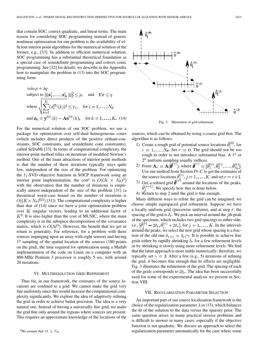See [32] for details; we describe in the Appendix how to manipulate the problem in (13) into the SOC program- ming form: subject to where and and for for (14) Fig. 3. Illustration of grid reﬁnement. For the numerical solution of our SOC problem, we use a package for optimization over self-dual homogeneous cones (which includes direct products of the positive orthant-con- straints, SOC constraints, and semideﬁnite cone constraints), called SeDuMi [33]. In terms of computational complexity, the interior point method relies on iterations of modiﬁed Newton’s method. One of the main attractions of interior point methods is that the number of these iterations typically stays quite low, independent of the size of the problem. For optimizing -SVD objective function in SOCP framework using an the interior point implementation, the cost8 is with the observation that the number of iterations is empir- ically almost independent of the size of the problem [31] (a theoretical worst-case bound on the number of iterations is [31]). The computational complexity is higher than that of [14] since we have a joint optimization problem over singular vectors, leading to an additional factor of . It is also higher than the cost of MUSIC, where the main complexity is in the subspace decomposition of the covariance matrix, which is . However, the beneﬁt that we get in return is generality. For reference, for a problem with three sources impinging upon an array with eight sensors and having 1 sampling of the spatial location of the sources (180 points on the grid), the time required for optimization using a Matlab implementation of the code on Linux on a computer with an 800-MHz Pentium 3 processor is roughly 5 sec, with around 20 iterations. VI. MULTIRESOLUTION GRID REFINEMENT Thus far, in our framework, the estimates of the source lo- cations are conﬁned to a grid. We cannot make the grid very ﬁne uniformly since this would increase the computational com- plexity signiﬁcantly. We explore the idea of adaptively reﬁning the grid in order to achieve better precision. The idea is a very natural one: Instead of having a universally ﬁne grid, we make the grid ﬁne only around the regions where sources are present. This requires an approximate knowledge of the locations of the 8We assume that M N . sources, which can be obtained by using a coarse grid ﬁrst. The algorithm is as follows. 1) Create a rough grid of potential source locations , for . The grid should not be too rough in order to not introduce substantial bias. A 1 or 2 uniform sampling usually sufﬁces. . Set 2) Form , where . Use our method from Section IV-C to get the estimates of the source locations . around the locations of the peaks, 3) Get a reﬁned grid , and set . We specify how this is done below. , for 4) Return to step 2 until the grid is ﬁne enough. Many different ways to reﬁne the grid can be imagined; we choose simple equispaced grid reﬁnement. Suppose we have a locally uniform grid (piecewise uniform), and at step , the spacing of the grid is . We pick an interval around the th peak of the spectrum, which includes two grid spacings to either side, i.e., . In the intervals around the peaks, we select the new grid whose spacing is a frac- tion of the old one . It is possible to achieve ﬁne grids either by rapidly shrinking for a few reﬁnement levels or by shrinking it slowly using more reﬁnement levels. We ﬁnd that the latter approach is more stable numerically; therefore, we typically set . After a few (e.g., 5) iterations of reﬁning the grid, it becomes ﬁne enough that its effects are negligible. Fig. 3 illustrates the reﬁnement of the grid. The spacing of each of the grids corresponds to . The idea has been successfully used for some of the experimental analysis we present in Sec- tion VIII. VII. REGULARIZATION PARAMETER SELECTION An important part of our source localization framework is the choice of the regularization parameter in (13), which balances the ﬁt of the solution to the data versus the sparsity prior. The same question arises in many practical inverse problems and is difﬁcult to answer in many cases, especially if the objective function is not quadratic. We discuss an approach to select the regularization parameter automatically for the case where some

3016 IEEE TRANSACTIONS ON SIGNAL PROCESSING, VOL. 53, NO. 8, AUGUST 2005 statistics of the noise are known or can be estimated. Let us as denote the estimate of the spatial spectrum obtained using the regularization parameter by . A well-known idea under the name of discrepancy principle [34] is to select to match the residuals of the solution to some known statistics of the noise when such are available. For example, if the distribution of is known or can be modeled, then one can select the noise . Here, the we use the . Directly searching for a to achieve the equality is rather difﬁcult and requires Frobenius norm value of solving the problem (13) multiple times for different such that vec s. Instead, we propose to look at the constrained version of the problem in (13), which can also be efﬁciently solved in the SOC framework [20]: subject to (15) vec . If distribution with has approximately a high enough so that the probability that The problem in (15) is equivalent via Lagrange multipliers to the one in (13) for some parameter , which is related to . For the problem in (15), the task of choosing the regulariza- tion parameter properly is considerably more transparent: We choose is small, where is independent and iden- tically distributed (i.i.d.) Gaussian, then for moderate to high SNR, de- grees of freedom upon normalization by the variance of . The reason that this holds only approximately is that the SVD in (10) depends on the particular re- alization of noise, and hence, the matrix is a function of . However, when noise is small, the term dominates the SVD, and the change due to the addition of is small, and we arrive at a . With the knowledge of the dis- and use tribution, we can ﬁnd a conﬁdence interval for its upper value as a choice for . In simulations we present in Section VIII, we ﬁnd that this procedure generates appropriate regularization parameter choices for our problem when noise is reasonably small. We also present some thoughts on how to extend the range of the applicability of the procedure to higher levels of noise by characterizing the distribution of for lower SNR. distribution for When noise statistics are not known, and no knowledge of the number of sources is available, the choice of the regularization parameter is a difﬁcult question. It has been approached in the inverse problem community by methods such as L-curve [35]. An attempt to apply the L-curve to a subset selection problem in noise has been made in [36], but the authors have to make an assumption that the SNR is approximately known. The choice of the regularization parameter when no knowledge of the noise or of the sources is available is still an open problem. VIII. EXPERIMENTAL RESULTS In this section, we present several experimental results for our -SVD source localization scheme. First, we compare the spectra of -SVD to those of MUSIC [3], beamforming [2], Capon’s method [4], and the beamspace method in [14] under various conditions. Next, we discuss and present results on regularization parameter selection. Then, we analyze empiri- cally the bias and variance properties of our method. 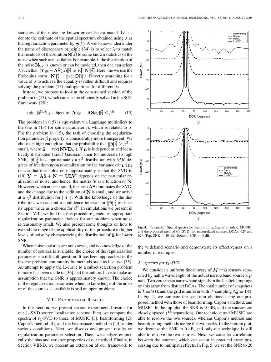Finally, in Section VIII-D, we present an extension of our framework to Fig. 4. (a) and (b). Spatial spectra for beamforming, Capon’s method, MUSIC, and the proposed method (` -SVD) for uncorrelated sources. DOAs: 62 and 67 . Top: SNR = 10 dB. Bottom: SNR = 0 dB. the wideband scenario and demonstrate its effectiveness on a number of examples. A. Spectra for -SVD We consider a uniform linear array of , and the grid is uniform with 1 sampling sensors sepa- rated by half a wavelength of the actual narrowband source sig- nals. Two zero-mean narrowband signals in the far-ﬁeld impinge on this array from distinct DOAs. The total number of snapshots is . In Fig. 4, we compare the spectrum obtained using our pro- posed method with those of beamforming, Capon’s method, and MUSIC. In the top plot, the SNR is 10 dB, and the sources are closely spaced (5 separation). Our technique and MUSIC are able to resolve the two sources, whereas Capon’s method and beamforming methods merge the two peaks. In the bottom plot, we decrease the SNR to 0 dB, and only our technique is still able to resolve the two sources. Next, we consider correlation between the sources, which can occur in practical array pro- cessing due to multipath effects. In Fig. 5, we set the SNR to 20

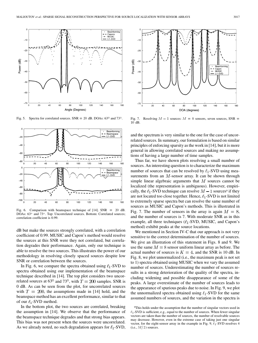
MALIOUTOV et al.: SPARSE SIGNAL RECONSTRUCTION PERSPECTIVE FOR SOURCE LOCALIZATION WITH SENSOR ARRAYS 3017 Fig. 5. Spectra for correlated sources. SNR = 20 dB. DOAs: 63 and 73 . Fig. 7. Resolving M 1 sources: M = 8 sensors, seven sources, SNR = 10 dB. and the spectrum is very similar to the one for the case of uncor- related sources. In summary, our formulation is based on similar principles of enforcing sparsity as the work in [14], but it is more general in allowing correlated sources and making no assump- tions of having a large number of time samples. Thus far, we have shown plots resolving a small number of sources. An interesting question is to characterize the maximum -SVD using mea- number of sources that can be resolved by surements from an -sensor array. It can be shown through simple linear algebraic arguments that sources cannot be localized (the representation is ambiguous). However, empiri- cally, the sources9 if they -SVD technique can resolve -SVD is not limited are not located too close together. Hence, to extremely sparse spectra but can resolve the same number of sources as MUSIC and Capon’s methods. This is illustrated in Fig. 7. The number of sensors in the array is again , and the number of sources is 7. With moderate SNR as in this example, all three techniques ( -SVD, MUSIC, and Capon’s method) exhibit peaks at the source locations. We mentioned in Section IV-C that our approach is not very sensitive to the correct determination of the number of sources. We give an illustration of this statement in Figs. 8 and 9. We use the same sensor uniform linear array as before. The actual number of sources is , and the SNR is 10 dB. In Fig. 8, we plot unnormalized (i.e., the maximum peak is not set to 1) spectra obtained using MUSIC when we vary the assumed number of sources. Underestimating the number of sources re- sults in a strong deterioration of the quality of the spectra, in- cluding widening and possible disappearance of some of the peaks. A large overestimate of the number of sources leads to the appearance of spurious peaks due to noise. In Fig. 9, we plot the unnormalized spectra obtained using -SVD for the same assumed numbers of sources, and the variation in the spectra is Fig. 6. Comparison with beamspace technique of [14]. SNR = 20 dB. DOAs: 63 and 73 . Top: Uncorrelated sources. Bottom: Correlated sources; correlation coefﬁcient is 0.99. dB but make the sources strongly correlated, with a correlation coefﬁcient of 0.99. MUSIC and Capon’s method would resolve the sources at this SNR were they not correlated, but correla- tion degrades their performance. Again, only our technique is able to resolve the two sources. This illustrates the power of our methodology in resolving closely spaced sources despite low SNR or correlation between the sources. In Fig. 6, we compare the spectra obtained using -SVD to spectra obtained using our implementation of the beamspace technique described in [14]. The top plot considers two uncor- related sources at 63 and 73 , with samples. SNR is 0 dB. As can be seen from the plot, for uncorrelated sources with , the assumptions made in [14] hold, and the beamspace method has an excellent performance, similar to that of our -SVD method. In the bottom plot, the two sources are correlated, breaking the assumption in [14]. We observe that the performance of the beamspace technique degrades and that strong bias appears. This bias was not present when the sources were uncorrelated. As we already noted, no such degradation appears for -SVD, 9This holds under the assumption that the number of singular vectors used in ` -SVD is sufﬁcient, e.g., equal to the number of sources. When fewer singular vectors are taken than the number of sources, the number of resolvable sources may decrease. However, even in the extreme case of taking just one singular vector, for the eight-sensor array in the example in Fig. 9, ` -SVD resolves 4 (i.e., M=2) sources.

分享到：

赞收藏

资料库

稀疏表示SAR成像.pdf

相关推荐

信息化

热门标签

最新资料