Engineering Structures 24 (2002) 1383–1396
www.elsevier.com/locate/engstruct
Path-dependent cyclic stress–strain relationship of reinforcing bar
including buckling
Rajesh Prasad Dhakal a,∗, Koichi Maekawa b
a Protective Technology Research Centre, School of Civil and Environmental Engineering, Nanyang Technological University, 50 Nanyang
b Department of Civil Engineering, The University of Tokyo, Hongo 7-3-1, Bunkyo-Ku, Tokyo 113-8656, Japan
Avenue, Singapore 639798
Received 25 January 2002; received in revised form 13 May 2002; accepted 21 May 2002
Abstract
In this paper, the formulation and verification of a cyclic stress–strain relationship of reinforcing bars are presented. The tension
envelope comprises an elastic range, a yield plateau and a hardening zone. The compression envelope also includes a linear elastic
range followed by a non-linear buckling model. The cyclic loops follow Giuffre–Menegotto–Pinto equations with some modifications
to account for the effect of buckling. A complete path-dependent cyclic constitutive model is then obtained by combining the
equations representing the two monotonic envelopes and the cyclic loops. Comparison with bare bar test results shows that the
proposed model could reasonably predict the cyclic behaviour of reinforcing bars including the post-buckling loops. 2002 Elsevier
Science Ltd. All rights reserved.
Keywords: Buckling; Reinforcing bar; Envelope; Cyclic loop; Path-dependent; Stress–strain relationship
1. Introduction
Although
As the performance-based design method is gaining
popularity, the reliable assessment of seismic perform-
ance has emerged as a vital step in seismic design. With
the advancement in computing facilities that can easily
handle complicated and large-scale mathematical oper-
ations, computational models with wider scope and
greater accuracy are being developed regardless of their
complexity.
on
member/component models can provide global structural
behaviour, constitutive models of constituent material
are needed to evaluate local response and also to assess
damage. An important constituent of reinforced concrete
(RC) members is the reinforcement, which has a domi-
nant contribution in the overall seismic response. Rein-
forcing bars inside RC structures experience a wide
range of strain variations when subjected to seismic exci-
tation. Apart from experiencing large tensile and com-
analysis
based
∗ Corresponding author. Tel.: +65-6790-4150; fax: +65-6791-0046.
E-mail address: cdhakal@ntu.edu.sg (R.P. Dhakal).
pressive strains, these bars also undergo random strain
reversals from different strain levels. As the post-elastic
response of reinforcing bars depends on strain history, a
reliable path-dependent cyclic stress–strain relationship
that can cover all possible strain paths is deemed neces-
sary for evaluating structural seismic performance ana-
lytically.
Some cyclic constitutive models for reinforcing bars
have been proposed recently. However, many of them
do not incorporate the effect of buckling [1–3]. Hence,
these models are applicable either to thick bars that are
unlikely to buckle within a reasonable compressive
strain range or to loading cases where strain does not
reach high values in compression. As buckling of rein-
forcing bars in RC members is not uncommon during
seismic excitations, proper consideration of buckling is
necessary for seismic performance evaluation, and mod-
els that ignore buckling are hence not ideal for use in
seismic analysis of RC structures. Buckling-induced
instability of reinforcing bars inside RC members has
been extensively studied in the past [4–9]. Some of these
studies also discussed the average compressive response
of reinforcing bars including buckling, but none came
up with a complete cyclic model. The authors are aware
0141-0296/02/$ - see front matter 2002 Elsevier Science Ltd. All rights reserved.
PII: S 0 1 4 1 - 02 96 ( 0 2 ) 0 0 08 0- 9
�
1384
R.P. Dhakal, K. Maekawa / Engineering Structures 24 (2002) 1383–1396
of a few cyclic models [10–12] that are reported to
include the effect of buckling.
the most
Rodriguez et al. [12] conducted monotonic and cyclic
tests on deformed steel bars. Based on test results of
several specimens, they proposed equations to locate
onset of buckling during monotonic and cyclic loadings.
They also proposed a cyclic constitutive model, which
is basically the same as that proposed by Mander et al.
[1] for cases without buckling with an additional rec-
ommendation to curtail the model at the onset of buck-
ling. Nevertheless, this model is silent on the post-buck-
ling response of reinforcing bars. Direct measurement of
steel stress inside RC columns [10] and cyclic tests on
bare bars [11] have shown that reinforcing bars can carry
significant tensile stress even after the initiation of buck-
ling, although the compressive stress-carrying capacity
decreases. One of
informative studies on
reinforcement buckling is that conducted by Suda et al.
[10], in which they monitored the stress carried by rein-
forcing bars
inside RC columns with a specially
designed stress sensor. With the help of these special
test results and some assumptions, they came up with a
cyclic stress–strain relationship of
reinforcing bars
including buckling. However, this relationship suggests
a common post-buckling behaviour for all bars regard-
less of their geometrical and mechanical properties. This
does not seem logical, as past studies [6,7,13] have
shown that the buckling initiation point and the post-
buckling response are sensitive to the bar length to bar
diameter ratio (i.e.
the slenderness ratio) and yield
strength of the bar. In another genuine effort, Monti and
Nuti [11] conducted monotonic and cyclic tests on some
normal-strength deformed steel bars, and concluded that
buckling takes place in bars only with slenderness ratio
greater than 5. Based on the test results, they proposed
equations to relate average compressive response with
the slenderness ratio. They also theoretically derived
equations for cyclic loops based on different hardening
rules for cases with and without buckling, and modified
an existing cyclic model [14] to represent results of the
tests that included buckling. However, the equations pro-
posed and the constants included were derived to fit the
test results of normal-strength bars (fy ⫽ 480 MPa) with
slenderness ratio equal
to 5, 8 and 11 only. Conse-
quently, these equations cannot be general as they cover
only a narrow range of geometrical properties and do
not take into account the effect of yield strength and
bar types.
This paper presents a path-dependent cyclic model for
reinforcing bars that overcomes the aforementioned
shortcomings. The model proposed here fulfils the fol-
lowing requirements: (1) it takes into account the effect
of geometrical and mechanical properties of the bar on
its post-buckling response, and is applicable to bars with
any material properties and any type of hardening mech-
anism; (2) it is of s ⫽ f(e) type, which offers significant
in any non-linear finite element
advantages
(FE)
computation based on kinematic approximations, as in
displacement-controlled FE analysis; (3) it is fully path-
dependent and covers all possible strain paths; and (4)
it is simple in formulation and is based on material para-
meters that are readily available, making it easy to
implement/encode into any FE analysis program.
2. Uniaxial monotonic curves
Manufacturers of reinforcing bars usually provide
mechanical properties that partly or completely define
the uniaxial tensile behaviour of their products. Never-
theless, values of these parameters in compression are
seldom specified,
thus implicitly compelling one to
assume that these properties are isotropic and are equal
in tension and compression. This is true when we talk
about the point-wise stress–strain relationships because
the point-wise relationships are not influenced by the
change in overall geometry [2]. On the other hand, aver-
age tensile and compressive behaviours are not necessar-
ily the same, as a geometrical non-linearity exists in
compression [13] due to lateral deformation of reinforc-
ing bars; referred to as buckling hereafter. As monotonic
compression test results [1,11] suggest that the average
compressive stress–strain curves of
reinforcing bar
samples with slenderness ratio small enough to avoid
premature buckling are very close to the corresponding
tension envelopes, it is assumed in this study that the
average compressive and tensile envelopes are similar in
the absence of buckling.
2.1. Tension envelope
Accurate representation of
the tension envelope
becomes indispensable to ensure the accuracy of the
complete cyclic model because both the compression
envelope and cyclic loops are influenced by the tension
envelope. Note that specifying only yield strength,
Young modulus and breaking strength does not com-
pletely describe the tensile response of a bar. To trace
the post-yielding tensile response until breaking, it is
necessary to specify the range of the yield plateau, the
nature of strain-hardening, the hardening stiffness, and
the breaking strain. The authors are of the view that it
is not appropriate to extrapolate the hardening behaviour
of a bar based on its elastic properties. Tensile properties
of deformed bars reported in Refs. [8,11,15,16] manifest
that the hardening behaviours of bars with different yield
strength and manufactured in different parts of the globe
are significantly different from one another. As the hard-
ening behaviour of deformed bars becomes more brittle
with increase in yield strength, normalizing the post-
yield tension parameters with respect to the yield stress
and yield strain cannot be justified. In order to generate
�
R.P. Dhakal, K. Maekawa / Engineering Structures 24 (2002) 1383–1396
1385
a universal cyclic model that can be used for bars with
any type of hardening behaviour, the complete tension
envelope is used as an input.
Regardless of the manufacturer and yield strength, the
tension envelope of all bars can be represented qualitat-
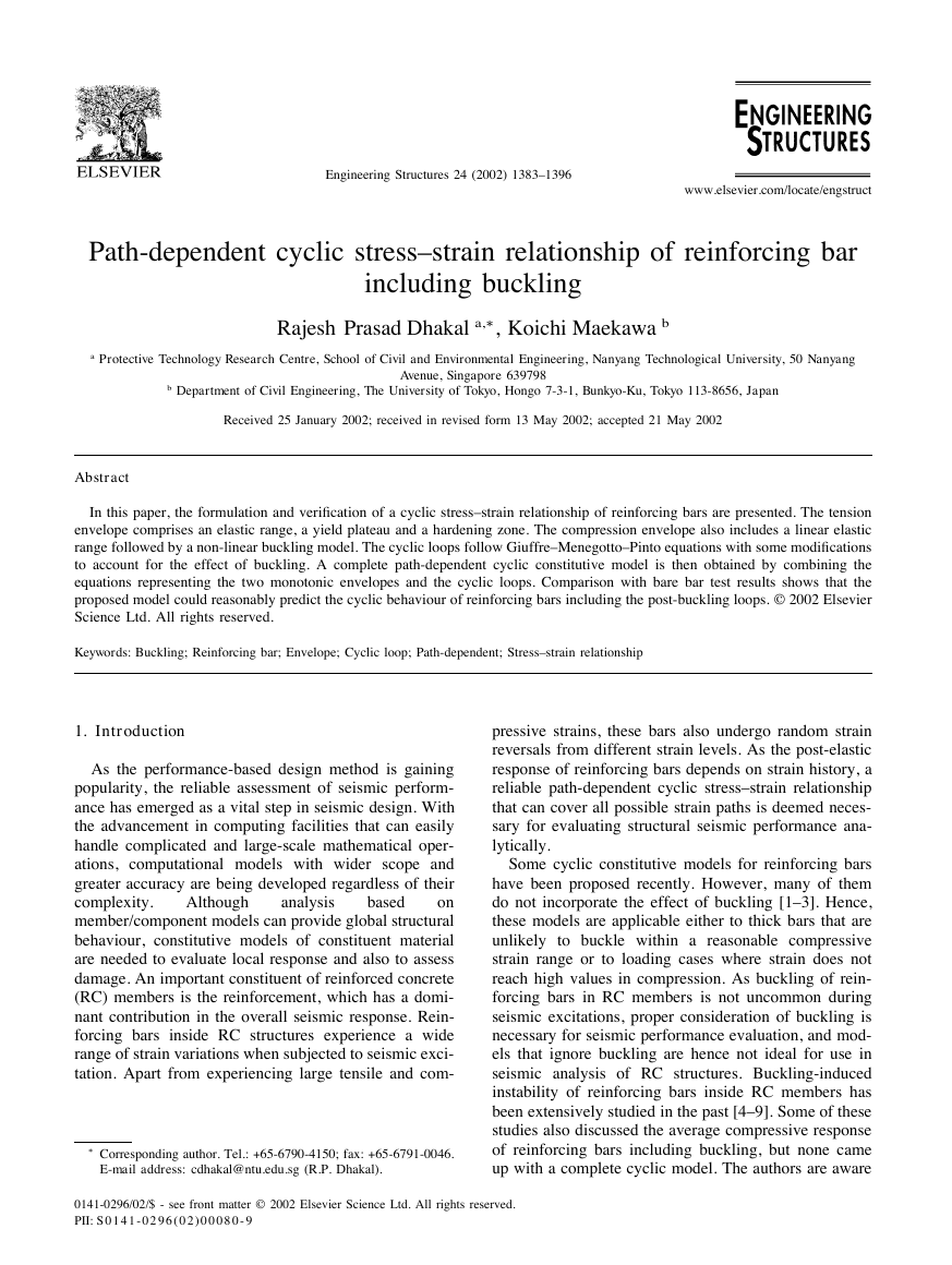
ively as shown in Fig. 1(a). The tension envelope con-
sists of four parts: an elastic branch (O–Y), a yield pla-
teau (Y–H), a strain-hardening zone (H–U) and the post-
ultimate descending branch (U–F). Although a closer
look inside the yield plateau is reported to reveal small
stress undulations [2], it is represented here as a straight
line with the stress equal to the yield strength for sim-
plicity. As the final post-ultimate descending branch is
of less significance in RC structural analysis, the tension
envelope only up to the ultimate stress point is usually
considered. The tension envelop until the strain-harden-
ing point esh can be represented by the following uniaxial
stress–strain (sst–est) relationships:
sst ⫽ Esest for estⱕey
and
sst ⫽ fy for ey ⬍ estⱕesh.
(2)
In Eqs. (1) and (2), Es, fy, ey and esh are Young’s
modulus, yield strength, yield strain and strain at the
starting point of hardening, respectively. Mander et al.
[1] proposed the following equations to idealize the non-
linear strain-hardening branch:
(1)
for esh ⬍ estⱕeu
冊P
sst ⫽ fu ⫹ (fy⫺fu)冉eu⫺est
P ⫽ Esh冉eu⫺esh
冊.
eu⫺esh
and
fu⫺fy
(3)
(4)
Here, fu and eu are respectively the stress and strain
at the ultimate point, and P is a parameter that describes
the shape of the hardening curve. P can be calculated as
shown in Eq. (4), where Esh is the tangential stiffness of
the hardening curve at the starting point. Note that P
equal to zero (i.e. Esh ⫽ 0) represents an elasto-plastic
bar, and P equal to 1 [i.e. Esh ⫽ (fu–fy) / (eu⫺esh)] rep-
resents a bar with linear strain-hardening behaviour.
Although the coordinates of the strain-hardening point
and the ultimate point can be located in an envelope, it
is not easy to measure Esh correctly. To avoid the uncer-
tainty involved in estimating Esh, Rodriguez et al. [12]
proposed the following equation that utilizes the coordi-
nates of any point (esh1, fsh1) in the strain-hardening zone
to evaluate P:
冊
log冉fu⫺fsh1
冊.
log冉eu⫺esh1
fu⫺fy
eu⫺esh
P ⫽
(5)
If the correct value of initial hardening stiffness Esh
is not known, the authors also prefer to use Eq. (5) as
it provides better control over the shape of the strain-
hardening curve. If an intermediate point is selected
properly, a bilinear approximation as shown in Fig. 1(b)
can also closely represent the hardening curve. However,
the selection of the intermediate point (esh1, fsh1) is diffi-
cult, when only the extreme points of the strain-harden-
ing curve are supplied and the nature of the hardening
curve in between is not known. In such cases, it is rec-
ommended to assume esh1 ⫽ [0.5(esh ⫹ eu)] and fsh1 ⫽
[fy ⫹ 0.75(fu–fy)].
2.2. Compression envelope
As mentioned earlier,
the average compressive
response within a control volume including the effect of
buckling is different from the tensile one, although the
point-wise stress–strain relationships in tension and
compression are the same regardless of buckling. In the
past, a few average compressive stress–strain relation-
ships including buckling have been proposed [11,12] to
satisfy the results of the tests, which were conducted
within a small range of slenderness ratio. Because of
the
different material properties used in these tests,
Fig. 1. Schematic representation of monotonic tension envelope.
�
1386
R.P. Dhakal, K. Maekawa / Engineering Structures 24 (2002) 1383–1396
empirical relationships derived differ considerably from
one another. Although the equations proposed could pre-
dict the effect of slenderness ratio in the tested range,
they do not account for the effect of other parameters
such as yield strength that was not varied in the tests. As
a general model has to cover conditions that are hardly
reproduced in the tests,
the experiments planned for
obtaining widely applicable constitutive models should
consist of test specimens that systematically cover a
wide range of geometrical as well as mechanical proper-
ties. Experiments consisting of a few specimens with
random properties are, of course, informative, and better
suited to verify proposed models rather than to generate
new models based on them.
In order to generate data for model formulation, the
authors conducted an analytical parametric study based
on the fibre technique [14], where the elements were
intentionally chosen to be of small length to ensure that
the behaviour within an element is unaffected by global
geometrical alterations. Hence, use of the tension envel-
ope to represent the compressive stress–strain relation-
ship of fibres in each element regardless of the extent of
buckling is justified. To reproduce actual test conditions,
rotation and displacement at the two extreme nodes were
restrained, and an axial downward displacement was
applied gradually at the topmost node. Of course, the
analytical tool was verified experimentally [13] before
conducting the extensive parametric study. Length L,
diameter D and yield strength fy of the bar were ident-
ified to govern the axial load–displacement relationship,
and these three parameters were varied within wide
ranges to investigate their effect on the average com-
pressive response.
Detailed discussions on the analytical method and the
results are beyond the scope of this paper, and have been
reported in another paper [13]. A typical result of the
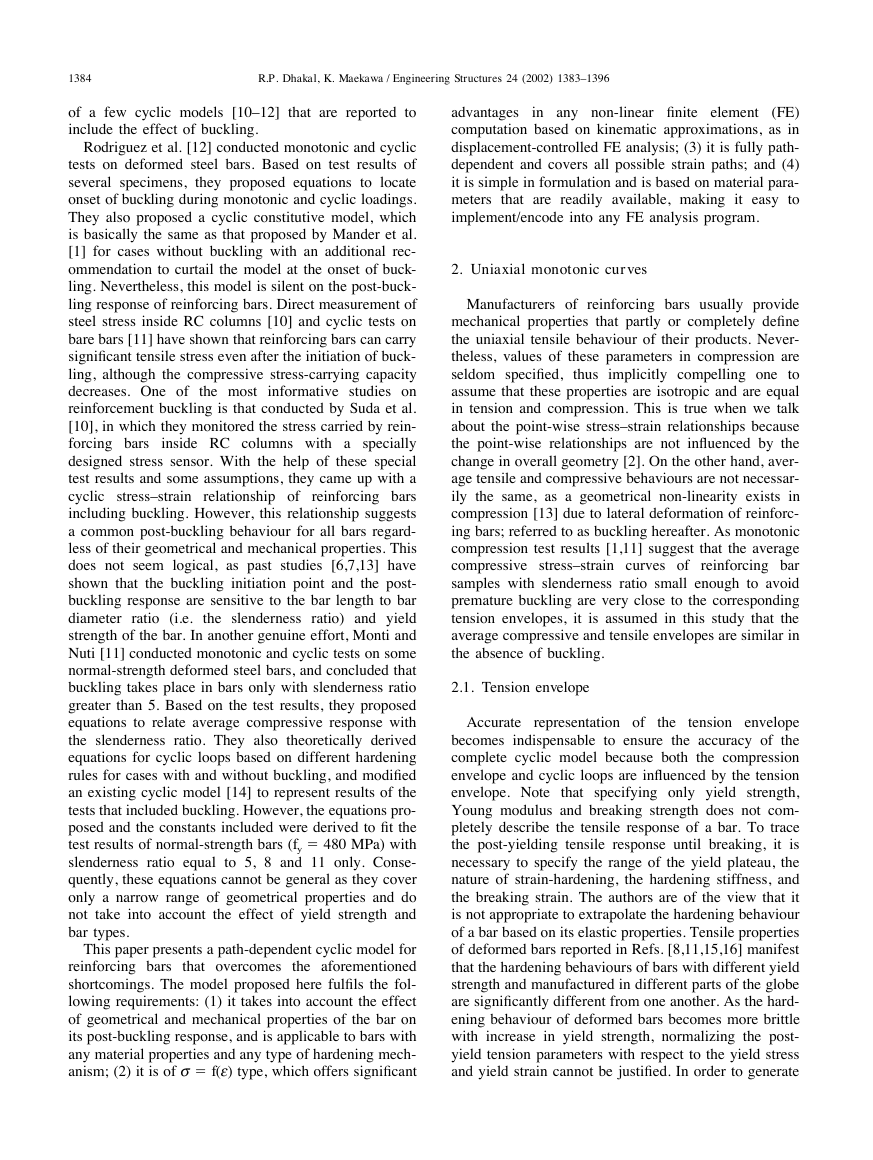
parametric study for an elastic–perfectly plastic bar is
illustrated in Fig. 2. The comparative normalized aver-
age stress–strain curves for slenderness ratios of 5 and
10 and yield strengths ranging from 100 MPa to 1600
MPa are presented in Fig. 2(a) and (b), respectively. The
results suggest that the critical slenderness ratio below
which the effect of buckling is negligible depends also
on yield strength of the reinforcing bar. Interestingly,
two pairs of special cases [(i) fy ⫽ 100 MPa, L/ D ⫽
10 and fy ⫽ 400 MPa, L/ D ⫽ 5;
fy ⫽
400 MPa, L/ D ⫽ 10 and fy ⫽ 1600 MPa, L / D ⫽ 5],
compared in Fig. 2(c), showed similar average responses
for the two cases in each pair, suggesting that the nor-
malized average compressive response depends only on
L/ D√fy. The variation of normalized compressive stress
with L / D√fy is shown in Fig. 2(d). As the value of
L/ D√fy increases,
the buckling-induced stress degra-
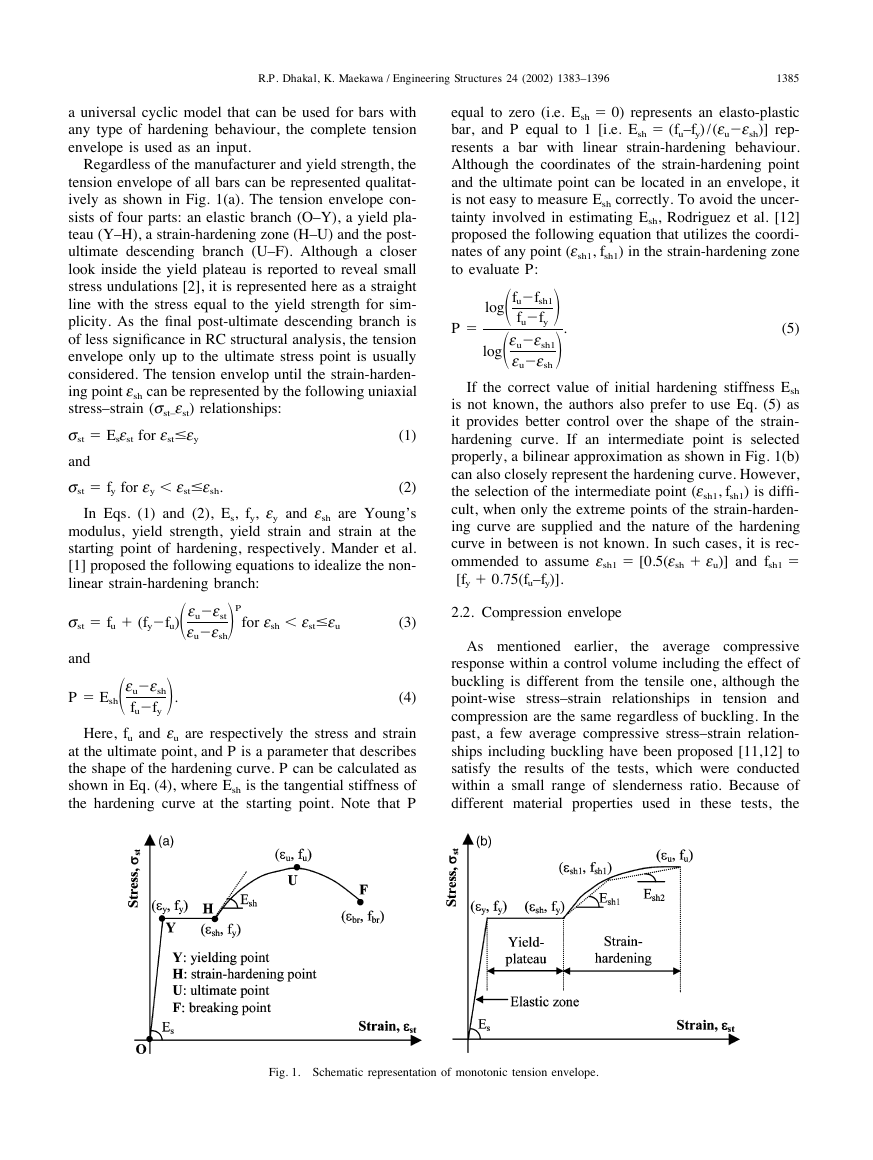
dation becomes more severe. Next, similar parametric
study was conducted for reinforcing bars with a linear
and (ii)
strain-hardening behaviour as shown in Fig. 3(a). The
normalized compressive stress–strain curves for these
bars with slenderness ratios ranging from 5 to 15 for
yield strengths equal to 200, 400 and 800 MPa are shown
in Fig. 3(b)–(d), respectively. In this case too, the aver-
age compressive response was found to depend uniquely
on L / D√fy, irrespective of separate values of L, D and
fy. The past studies could not unearth this unique inter-
relationship, which is the backbone of the model pro-
posed in this paper.
Through this analytical parametric study, various facts
regarding the average behaviour of reinforcing bars in
compression are revealed. Some of them are: (1) the
average compressive stress–strain relationship can be
described completely by L / D√fy; (2) the average com-
pression envelope lies below the tension envelope when
plotted together; (3) the trend of average compressive
stress degradation depends on the value of L/ D√fy and
also on the tension envelope; (4) regardless of L/ D√fy,
the compressive stress degradation rate in the later stage
is nearly constant with a negative slope approximately
equal to 0.02Es; and (5) the average compressive stress
becomes constant after it becomes equal to 20% of the
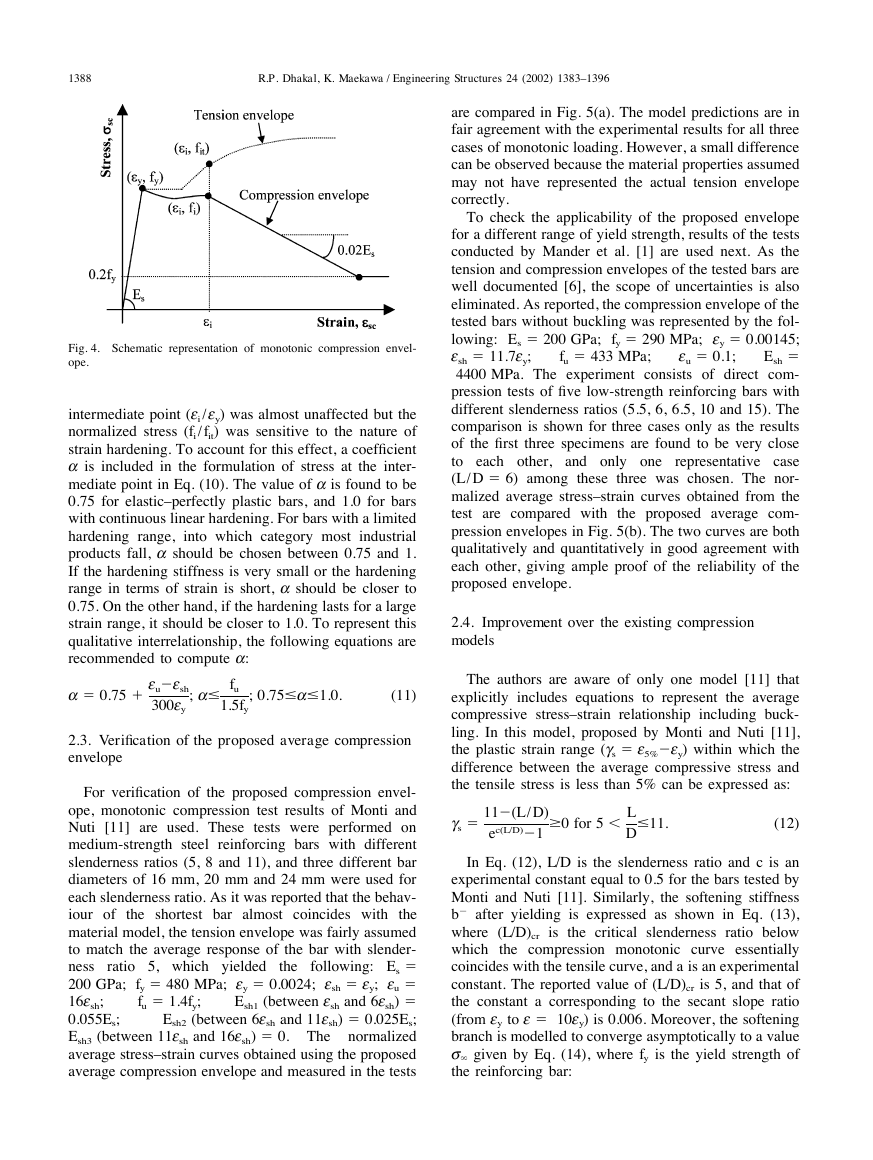
yield strength. Guided by these unique interrelationships,
an
stress–strain
relationship is proposed, the general layout of which is
sketched in Fig. 4. Note that the compressive stresses
and strains specified in Fig. 4 and used in the equations
to follow are absolute, and their signs should be changed
before merging with
and
unloading/reloading loops to form a complete cyclic
model. An intermediate point (ei, fi) is established, after
which a constant negative stiffness equal to 0.02Es is
applied until the average compressive stress becomes
equal to 0.2fy. To represent the aforementioned mech-
anisms, the following compressive stress–strain (ssc–esc)
relationships are proposed:
ssc ⫽ Esesc for escⱕey,
average monotonic
compressive
envelope
tension
the
(6)
⫽ 1⫺冉1⫺fi
冊冉esc⫺ey
冊 for ey ⬍ escⱕei
fit
(7)
ei⫺ey
ssc
st
and
ssc ⫽ fi⫺0.02Es(esc⫺ei); sscⱖ0.2fy for esc ⬎ ei.
(8)
Here, st and fit are the stresses in the tension envelope
corresponding to esc (current strain) and ei (strain at the
intermediate point), respectively. To make the model
applicable to bars with all types of material model, the
compressive stress ssc at and before the intermediate
point is normalized with respect to st. This normaliz-
ation technique also renders the shape of the average
compression envelope before this intermediate point
look like the tension envelope; a characteristic that was
observed distinctly in all analytical results. The coordi-
nates of intermediate points in the analytically generated
�
R.P. Dhakal, K. Maekawa / Engineering Structures 24 (2002) 1383–1396
1387
Fig. 2. Average compressive responses of elastic–perfectly plastic bars.
Fig. 3. Average compressive responses of bars with strain hardening.
average compression envelopes could be correlated to
L/ D√fy as:
⫽ 55⫺2.3冪 fy
ei
ey
and
ei
ey
100
L
D
;
ⱖ7
(9)
fi
fit
⫽ a冉1.1⫺0.016冪 fy
100
冊;
fi
fy
ⱖ0.2.
(10)
L
D
Comparison between the average compression envel-
opes of the elastic–perfectly plastic and the linear strain-
hardening bars revealed that the normalized strain at the
�
1388
R.P. Dhakal, K. Maekawa / Engineering Structures 24 (2002) 1383–1396
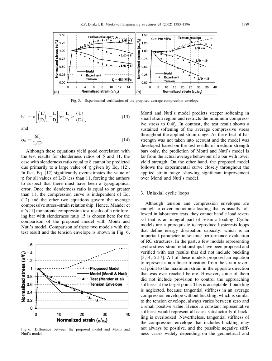
are compared in Fig. 5(a). The model predictions are in
fair agreement with the experimental results for all three
cases of monotonic loading. However, a small difference
can be observed because the material properties assumed
may not have represented the actual tension envelope
correctly.
eu ⫽ 0.1;
fu ⫽ 433 MPa;
To check the applicability of the proposed envelope
for a different range of yield strength, results of the tests
conducted by Mander et al. [1] are used next. As the
tension and compression envelopes of the tested bars are
well documented [6], the scope of uncertainties is also
eliminated. As reported, the compression envelope of the
tested bars without buckling was represented by the fol-
lowing: Es ⫽ 200 GPa;
fy ⫽ 290 MPa; ey ⫽ 0.00145;
esh ⫽ 11.7ey;
Esh ⫽
4400 MPa. The experiment consists of direct com-
pression tests of five low-strength reinforcing bars with
different slenderness ratios (5.5, 6, 6.5, 10 and 15). The
comparison is shown for three cases only as the results
of the first three specimens are found to be very close
to each other, and only one representative case
(L / D ⫽ 6) among these three was chosen. The nor-
malized average stress–strain curves obtained from the
test are compared with the proposed average com-
pression envelopes in Fig. 5(b). The two curves are both
qualitatively and quantitatively in good agreement with
each other, giving ample proof of the reliability of the
proposed envelope.
2.4. Improvement over the existing compression
models
The authors are aware of only one model [11] that
explicitly includes equations to represent the average
compressive stress–strain relationship including buck-
ling. In this model, proposed by Monti and Nuti [11],
the plastic strain range (gs ⫽ e5%⫺ey) within which the
difference between the average compressive stress and
the tensile stress is less than 5% can be expressed as:
gs ⫽ 11⫺(L / D)
ec(L/D)⫺1
ⱖ0 for 5 ⬍ L
D
ⱕ11.
(12)
In Eq. (12), L/D is the slenderness ratio and c is an
experimental constant equal to 0.5 for the bars tested by
Monti and Nuti [11]. Similarly, the softening stiffness
b⫺ after yielding is expressed as shown in Eq. (13),
is the critical slenderness ratio below
where (L/D)cr
which the compression monotonic curve essentially
coincides with the tensile curve, and a is an experimental
constant. The reported value of (L/D)cr is 5, and that of
the constant a corresponding to the secant slope ratio
(from ey to e ⫽ 10ey) is 0.006. Moreover, the softening
branch is modelled to converge asymptotically to a value
s⬁ given by Eq. (14), where fy is the yield strength of
the reinforcing bar:
Fig. 4. Schematic representation of monotonic compression envel-
ope.
intermediate point (ei /ey) was almost unaffected but the
normalized stress (fi/ fit) was sensitive to the nature of
strain hardening. To account for this effect, a coefficient
a is included in the formulation of stress at the inter-
mediate point in Eq. (10). The value of a is found to be
0.75 for elastic–perfectly plastic bars, and 1.0 for bars
with continuous linear hardening. For bars with a limited
hardening range, into which category most industrial
products fall, a should be chosen between 0.75 and 1.
If the hardening stiffness is very small or the hardening
range in terms of strain is short, a should be closer to
0.75. On the other hand, if the hardening lasts for a large
strain range, it should be closer to 1.0. To represent this
qualitative interrelationship, the following equations are
recommended to compute a:
a ⫽ 0.75 ⫹ eu⫺esh
; aⱕ fu
300ey
1.5fy
; 0.75ⱕaⱕ1.0.
(11)
2.3. Verification of the proposed average compression
envelope
For verification of the proposed compression envel-
ope, monotonic compression test results of Monti and
Nuti [11] are used. These tests were performed on
medium-strength steel reinforcing bars with different
slenderness ratios (5, 8 and 11), and three different bar
diameters of 16 mm, 20 mm and 24 mm were used for
each slenderness ratio. As it was reported that the behav-
iour of
the shortest bar almost coincides with the
material model, the tension envelope was fairly assumed
to match the average response of the bar with slender-
ratio 5, which yielded the following: Es ⫽
ness
fy ⫽ 480 MPa; ey ⫽ 0.0024; esh ⫽ ey; eu ⫽
200 GPa;
fu ⫽ 1.4fy;
Esh1 (between esh and 6esh) ⫽
16esh;
Esh2 (between 6esh and 11esh) ⫽ 0.025Es;
0.055Es;
Esh3 (between 11esh and 16esh) ⫽ 0. The
normalized
average stress–strain curves obtained using the proposed
average compression envelope and measured in the tests
�
R.P. Dhakal, K. Maekawa / Engineering Structures 24 (2002) 1383–1396
1389
Fig. 5. Experimental verification of the proposed average compression envelope.
⬎冉L
冊
D
cr
冊
⫺L
D
cr
册for
L
D
b⫺ ⫽ a冋冉L
D
and
s⬁ ⫽ 6fy
L/ D
.
(13)
(14)
Although these equations yield good correlation with
the test results for slenderness ratios of 5 and 11, the
case with slenderness ratio equal to 8 cannot be predicted
due primarily to a large value of gs given by Eq. (12).
In fact, Eq. (12) significantly overestimates the value of
gs for all values of L/D less than 11, forcing the authors
to suspect that there must have been a typographical
error. Once the slenderness ratio is equal to or greater
than 11, the compression curve is independent of Eq.
(12) and the other two equations govern the average
compressive stress–strain relationship. Hence, Mander et
al’s [1] monotonic compression test results of a reinforc-
ing bar with slenderness ratio 15 is chosen here for the
comparison of the proposed model with Monti and
Nuti’s model. Comparison of these two models with the
test result and the tension envelope is shown in Fig. 6.
Fig. 6. Difference between the proposed model and Monti and
Nuti’s model.
Monti and Nuti’s model predicts steeper softening in
small strain region and restricts the minimum compress-
ive stress to 0.4fy. In contrast, the test result shows a
sustained softening of the average compressive stress
throughout the applied strain range. As the effect of bar
strength was not taken into account and the model was
developed based on the test results of medium-strength
bars only, the prediction of Monti and Nuti’s model is
far from the actual average behaviour of a bar with lower
yield strength. On the other hand, the proposed model
follows the experimental curve closely throughout the
applied strain range, showing significant improvement
over Monti and Nuti’s model.
3. Uniaxial cyclic loops
Although tension and compression envelopes are
enough to cover monotonic loading that is usually fol-
lowed in laboratory tests, they cannot handle load rever-
sal that is an integral part of seismic loading. Cyclic
models are a prerequisite to reproduce hysteresis loops
that define energy dissipation capacity, which is an
important parameter in seismic performance evaluation
of RC structures. In the past, a few models representing
cyclic stress–strain relationships have been proposed and
verified with test results that did not include buckling
[3,14,15,17]. All of these models proposed an equation
to represent a non-linear transition from the strain-rever-
sal point to the maximum strain in the opposite direction
that was ever reached before. However, some of them
did not include provision to control the approaching
stiffness at the target point. This is acceptable if buckling
is neglected, because tangential stiffness in an average
compression envelope without buckling, which is similar
to the tension envelope, always varies between zero and
a small positive value. Hence, a constant representative
stiffness would represent all cases satisfactorily if buck-
ling is overlooked. Nevertheless, tangential stiffness of
the compression envelope that includes buckling may
not always be positive, and the possible negative stiff-
ness varies widely depending on the geometrical and
�
1390
R.P. Dhakal, K. Maekawa / Engineering Structures 24 (2002) 1383–1396
mechanical properties of the bar. A negative stiffness at
the minimum strain point may generate an unloading
curve that shows compressive stress reduction even
before entering the compressive strain zone. This tend-
ency in the cyclic loops can be simulated only if the
stiffness at the target point is also taken into account
in formulating the trajectory of the loop. Therefore, the
Giuffre–Menegotto–Pinto model [18] that satisfies the
aforementioned condition is adopted in this study, and
some modifications are made to account for the effects
of buckling.
3.1. Original Giuffre–Menegotto–Pinto model
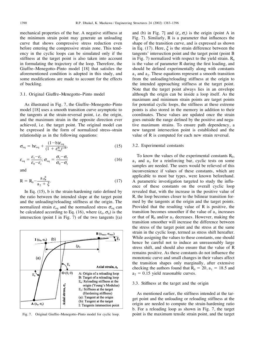
As illustrated in Fig. 7, the Giuffre–Menegotto–Pinto
model [18] uses a smooth transition curve asymptotic to
the tangents at the strain-reversal point, i.e. the origin,
and the maximum strain in the opposite direction ever
achieved, i.e. the target point. The original model can
be expressed in the form of normalized stress–strain
relationship as in the following equations:
seq ⫽ beeq ⫹ (1⫺b)eeq
eq)1/R,
(1 ⫹ eR
; seq ⫽ ss⫺sr
s0⫺sr
eeq ⫽ es⫺er
e0⫺er
(15)
(16)
and
R ⫽ R0⫺ a1x
a2 ⫹ x
.
(17)
In Eq. (15), b is the strain-hardening ratio defined by
the ratio between the intended slope at the target point
and the unloading/reloading stiffness at the origin. The
normalized strain eeq and the normalized stress seq can
be calculated according to Eq. (16), where (e0, s0) is the
intersection (point I in Fig. 7) of the two tangents [(a)
Fig. 7. Original Giuffre–Menegotto–Pinto model for cyclic loop.
and (b) in Fig. 7] and (er, sr) is the origin (point A in
Fig. 7). Similarly, R is a parameter that influences the
shape of the transition curve, and is expressed as shown
in Eq. (17). Here, x is the strain difference between the
tangents’ intersection point and the target point (point B
in Fig. 7) normalized with respect to the yield strain. R0
is the value of parameter R during the first loading, and
should be defined experimentally along with constants
a1 and a2. These equations represent a smooth transition
from the unloading/reloading stiffness at the origin to
the intended approaching stiffness at the target point.
Note that the target point always lies in an envelope
although the origin can be inside a loop itself. As the
maximum and minimum strain points are target points
for potential cyclic loops, the stiffness at these extreme
points is also stored in the memory in addition to their
coordinates. These values are updated once the strain
goes outside the range defined by the positive and nega-
tive maximum strains. To ensure path dependency, a
new tangent intersection point is established and the
value of R is computed for each new strain reversal.
3.2. Experimental constants
To know the values of the experimental constants R0,
a1 and a2 for a reinforcing bar, cyclic tests on some
samples are needed. The users would be relieved of this
inconvenience if values of these constants, which are
applicable to most bar types, were known beforehand.
A parametric investigation targeted to study the influ-
ence of these constants on the overall cyclic loop
revealed that, with the increase in the positive value of
R, the loop becomes closer to the bilinear transition for-
med by the tangents at the origin and the target points.
Provided that the resulting value of R is positive, the
transition becomes smoother if the value of a1 increases
or that of R0 and/or a2 decreases. However, making the
transition smoother will increase the difference between
the stress of the target point and the stress at the same
strain in the cyclic loop, termed as stress shift hereafter.
While assigning the values to these constants, one should
hence be careful not to induce an unreasonably large
stress shift, and should also ensure that the value of R
remains positive. As these constants do not influence the
monotonic curve and small changes in their values affect
the transition shapes only marginally, after extensive
checking the authors found that R0 ⫽ 20, a1 ⫽ 18.5 and
a2 ⫽ 0.15 yield reasonable curves.
3.3. Stiffness at the target and the origin
As mentioned earlier, the stiffness intended at the tar-
get point and the unloading or reloading stiffness at the
origin are needed to compute the strain-hardening ratio
b. For a reloading loop as shown in Fig. 7, the target
point is the maximum tensile strain point, and the target
�



 2023年江西萍乡中考道德与法治真题及答案.doc
 2012年重庆南川中考生物真题及答案.doc
 2013年江西师范大学地理学综合及文艺理论基础考研真题.doc
 2020年四川甘孜小升初语文真题及答案I卷.doc
 2020年注册岩土工程师专业基础考试真题及答案.doc
 2023-2024学年福建省厦门市九年级上学期数学月考试题及答案.doc
 2021-2022学年辽宁省沈阳市大东区九年级上学期语文期末试题及答案.doc
 2022-2023学年北京东城区初三第一学期物理期末试卷及答案.doc
 2018上半年江西教师资格初中地理学科知识与教学能力真题及答案.doc
 2012年河北国家公务员申论考试真题及答案-省级.doc
 2020-2021学年江苏省扬州市江都区邵樊片九年级上学期数学第一次质量检测试题及答案.doc
 2022下半年黑龙江教师资格证中学综合素质真题及答案.doc