格兰杰因果分析工具箱介绍（MVGC）.pdf-资料库

Journal of Neuroscience Methods 223 (2014) 50– 68 Contents lists available at ScienceDirect Journal of Neuroscience Methods j o u r n a l h o m e p a g e : w w w . e l s e v i e r . c o m / l o c a t e / j n e u m e t h Computational Neuroscience The MVGC multivariate Granger causality toolbox: A new approach to Granger-causal inference Lionel Barnett∗, Anil K. Seth Sackler Centre for Consciousness Science and School of Informatics, University of Sussex, Brighton BN1 9QJ, UK h i g h l i g h t s • Matlab© Toolbox for accurate and efﬁcient calculation of Granger causality. • Calculate Granger causalities (conditional and unconditional) in both time and frequency domains. • Based on advanced VAR (vector autoregression) theory. • Avoids separate “full” and “reduced” regressions. a r t i c l e i n f o a b s t r a c t Article history: Received 5 September 2013 Received in revised form 16 October 2013 Accepted 26 October 2013 Keywords: Granger causality Vector autoregressive modelling Time series analysis 1. Introduction causality (G-causality) Wiener–Granger (Granger, 1969; Geweke, 1982, 1984) is an increasingly popular method for identi- fying “causal” connectivity in neural time series data (Bressler and Seth, 2011). It can be traced conceptually to Wiener (1956) and was operationalised by Granger in terms of linear autoregressive ∗ Corresponding author. Tel.: +44 1273 678101. E-mail addresses: l.c.barnett@sussex.ac.uk (L. Barnett), a.k.seth@sussex.ac.uk (A.K. Seth). 0165-0270/$ – see front matter © http://dx.doi.org/10.1016/j.jneumeth.2013.10.018 2013 Elsevier B.V. All rights reserved. Background: Wiener–Granger causality (“G-causality”) is a statistical notion of causality applicable to time series data, whereby cause precedes, and helps predict, effect. It is deﬁned in both time and frequency domains, and allows for the conditioning out of common causal inﬂuences. Originally developed in the context of econometric theory, it has since achieved broad application in the neurosciences and beyond. Prediction in the G-causality formalism is based on VAR (vector autoregressive) modelling. New method: The MVGC Matlab© Toolbox approach to G-causal inference is based on multiple equiva- lent representations of a VAR model by (i) regression parameters, (ii) the autocovariance sequence and (iii) the cross-power spectral density of the underlying process. It features a variety of algorithms for moving between these representations, enabling selection of the most suitable algorithms with regard to computational efﬁciency and numerical accuracy. Results: In this paper we explain the theoretical basis, computational strategy and application to empirical G-causal inference of the MVGC Toolbox. We also show via numerical simulations the advantages of our Toolbox over previous methods in terms of computational accuracy and statistical inference. Comparison with existing method(s): The standard method of computing G-causality involves estimation of parameters for both a full and a nested (reduced) VAR model. The MVGC approach, by contrast, avoids explicit estimation of the reduced model, thus eliminating a source of estimation error and improving statistical power, and in addition facilitates fast and accurate estimation of the computationally awkward case of conditional G-causality in the frequency domain. Conclusions: The MVGC Toolbox implements a ﬂexible, powerful and efﬁcient approach to G-causal inference. © 2013 Elsevier B.V. All rights reserved. modelling of stochastic processes (Granger, 1969). G-causality is based on predictability and precedence. Put simply, a variable X is said to G-cause a variable Y if the past of X contains information that helps predict the future of Y over and above information already in the past of Y. Importantly, G-causality is a measure of directed functional connectivity in terms of providing a statistical descrip- tion of observed responses. In contrast, methods for identifying effective connectivity aim to elucidate the “the simplest possible circuit diagram explaining observed responses” (Valdes-Sosa et al., 2011; Aertsen and Preißl, 1991; Friston et al., 2003, 2013). The MVGC Matlab Toolbox implements numerical routines for calculating multivariate Granger causality (MVGC) from time series

L. Barnett, A.K. Seth / Journal of Neuroscience Methods 223 (2014) 50– 68 51 data, both unconditional and conditional, in the time and frequency domains. It supersedes and extends the GCCA (Granger Causal Con- nectivity Analysis) Toolbox (Seth, 2010). Based on advanced VAR (vector autoregressive) model theory (Hamilton, 1994; Lütkepohl, 2005), it is designed for computational efﬁciency and accuracy. Improving upon standard approaches to G-causal inference, it avoids separate full and reduced regressions (see Section 2), thus eliminating a common source of statistical inaccuracy and computational inefﬁciency. It also facilitates estimation of fully multivariate conditional G-causality in the frequency domain. The MVGC toolbox has been designed with application to empir- ical neuroscience data in mind. Several issues commonly faced in applying G-causal inference to such data are discussed later in the paper (Section 4). However, the software is not restricted to this application domain. G-causal inference is a very general method which has been productively applied in many areas, though caution is always needed in ensuring that the data satisfy the assump- tions underpinning the method (see Section 2.1 and also Section 3.3). Thus, while the MVGC software is designed to be intuitive and straightforward to use, to get the most out of it some under- standing of the theoretical basis of G-causal inference, as well as approaches to its numerical computation, is recommended. To facilitate this, this paper presents the conceptual and theoretical basis of G-causality (substantially extending previous presenta- tions), and details the computational implementation of the MVGC toolbox. Although not intended as a user guide—the integrated help system and walk-through demonstration scripts fulﬁll that purpose—Section 3 provides a helpful overview of the toolbox rationale and design principles, Section 3.1 explains the MVGC computational strategy while Appendices A.1 and A.2 detail the core computational algorithms. 2. G-causality: theory, estimation and inference Y Y Y X X = Y 1, X1, X2, . . ., Y; intuitively, past values of X = X if and only if does convey information about the future of Assume two jointly distributed vector-valued stochastic pro- Y 2, . . .. We say that cesses (“variables”) Y X, conditional on its own past, does not G-cause yield is independent of the past of no information about the current value of beyond information itself. If, conversely, the past already contained in the past of of above and then we say that beyond all information contained in the past of Y X. Much has been made of the fact that this notion of “causality” does not necessarily tally with more conventional (and perhaps more physically intuitive) notions (Pearl, 2009; Valdes- Sosa et al., 2011; Friston, 2011; Roebroeck et al., 2009, 2010) (note, for example, that the processes must be strictly non-deterministic for the above deﬁnition even to make sense). We do not engage this debate here; throughout this paper the term “causal” is used exclusively in the Wiener–Granger sense just described. G-causes X X Testing for Granger (non-)causality requires establishing—in a statistical sense—a conditional (non-)dependency. This may seem to invite an information-theoretic approach, since mutual information is a natural measure of statistical dependence. How- ever in empirical settings a drawback with information-theoretic quantities is the difﬁculty of estimation in sample and lack of known theoretical distributions for information-theoretic esti- mators, complicating statistical inference (but see Barnett and Bossomaier, 2013). An alternative is therefore to invoke a model- based or parametric approach for which conditional dependency estimators are more efﬁcient and (preferably) have known samp- ling distributions, thus facilitating inference. In fact, G-causality is frequently identiﬁed with a model-based viewpoint, which may also yield intuitive predictive interpretations of G-causality; for X, conditional on its own past, predictive models, the statement “ is independent of the past of X Y predicted by its own past”. does not help predict Y” may be reframed as “the past of may be beyond the degree to which X The most common operationalisation of G-causality, and the one on which the MVGC Toolbox is based, utilises VAR modelling of time um, where for series data. A multivariate time series ut is a real-valued n-dimensional (column) vector with each time t components u1t, u2t, . . ., unt, is considered as a realisation of length m of a discrete-time stationary1 vector stochastic process U2, . . . (the “universe of variables”). A pth order vector autoregressive model for the process—a VAR(p)—takes the form2 u2, . . ., U1, u1, U t = Ak · U t−k + εt (1) p k=1 × Here p is the model order, which may be inﬁnite. The n n real-valued matrices Ak are the regression coefﬁcients, and the εt the residuals, which are n-dimensional stochastic process independently and identically distributed (iid) and serially uncor- is, they constitute a white noise process. The related; that × parameters of the model are the coefﬁcients Ak and the n n resid- ≡ cov(εt) which, by stationarity, does not uals covariance matrix depend on the time t. Interpreted as a predictive model, (1) thus models the value of the process at current time t in terms of its − past values at times t p. The regression coefﬁcients represent the predictable structure of the data, the residuals the unpredictable. − 1, . . ., t The determination of a VAR model (1) should not be taken to imply that the time series data modelled by the stochastic pro- ut was actually generated by a linear autoregressive scheme. cess In comparison to effective connectivity techniques like dynamic causal modelling [DCM] (Friston et al., 2003), which make very explicit assumptions about the generative mechanism underlying the observed data (Friston et al., 2013), the VAR models underlying G-causality are “generic”, in the sense that they make no assump- tions about the mechanism that produced the data, beyond that a VAR model actually exists. Standard theory (Anderson, 1971) yields that a rather general class of covariance-stationary multivariate process—including many nonlinear processes—may be modelled as VARs, albeit of theoretically inﬁnite order (see also the next section). Note that this belies a common misapprehension that VAR-based G-causal analysis is restricted to linear processes. In practice, given empirical time-series data, a ﬁnite model order p is selected on theoretical principles, sufﬁciently high so as to cap- ture predictable variation but not so high as to overﬁt unpredictable variation in the data (Section 2.4). 2.1. VAR process theory The MVGC toolbox exploits some advanced aspects of VAR pro- cess theory, which we outline here. For valid G-causality analysis, the VAR coefﬁcients in (1) must be square summable and stable (Hamilton, 1994; Lütkepohl, 2005; ∞ Rozanov, 1967). Square summability requires that Ak2 < p k=1 1 G-causal inference is not necessarily limited to stationary processes. Under some circumstances—notably for multi-trial data or for near-stationary data that may be “windowed”—the stationarity requirement may be relaxed. This is addressed later on. 2 Throughout, bold symbols represent vector quantities and normal typeface represents scalar quantities. Capitalised symbols represent random variables or U t for the random vector representing matrices, according to context. Thus we write U 2, . . . at time t, um for a realisation of the pro- u1, . . ., the value of the process ut, etc. A superscript cess of length m, uit for the ith component of denotes matrix ∗ transpose, and a superscript denotes (complex) matrix conjugate-transpose. |M| denotes the determinant of the square matrix M. U 1,

52 L. Barnett, A.K. Seth / Journal of Neuroscience Methods 223 (2014) 50– 68 For a VAR process, the CPSD admits a unique spectral factorisation (Papoulis and Pillai, 2002) ≤ ∗ = H()H() S() 0 ≤ 2 (9) where the transfer function H() is deﬁned as the inverse matrix of the Fourier transform of the regression coefﬁcients: (2) ≡ H() − I −ik Ake ≤ ≤ 2 0 (10) −1 p k=1 which means intuitively that the coefﬁcients do not “blow up” even for inﬁnite model order p (for ﬁnite p square summability is sat- isﬁed trivially). Stability means that the VAR coefﬁcients deﬁne a covariance-stationary process. This is related to the the characteristic polynomial for the coefﬁcients sequence Ak, which is: I p Akzk k=1 ≡ ϕA(z) − for the variable z deﬁned in the complex plane C. By standard the- ory (Lütkepohl, 2005) the coefﬁcients Ak deﬁne a stable VAR iff the ≤ characteristic polynomial is invertible on the unit disc |z| 1 in the complex plane. Deﬁning the spectral radius of the VAR as (A) ≡ max ϕA(z)=0 {|z|−1} (3) an equivalent condition covariance-stationary process—is for stability—i.e. that (1) deﬁne a (A) < 1 (4) −2, cov(ut, = . . ., ut−k) k −1, 0, 1, 2, . . . The autocovariance sequence k for a covariance-stationary (not ut is deﬁned as the sequence necessarily VAR) stochastic process × of n n matrices k ≡ Note that by stationarity the k do not depend on the time t, and for all lags k. For a VAR process of the form (1), it may that −k = k be shown [Appendix A.1, (A5)] that in the long run, the autocovari- ance sequence decays exponentially with lag k, the rate of decay being just the spectral radius (A). Note, importantly, that this implies that if the autocovariance sequence for a process does not decay (sub-)exponentially then the process may not be modelled as a VAR (see Section 3.3). This has some importance for analysis of neural data, which we return to in Section 4.2. (5) For a VAR process (1), the autocovariance sequence is related to the VAR parameters via the Yule-Walker equations (Anderson, 1971) k = Ak− + ık0 k = . . ., −2, −1, 0, 1, 2, . . . (6) p =1 Numerically, there are efﬁcient algorithms available for solving (6) for the k in terms of (Ak, ) [Appendix A.1, (A5)] and, conversely, for (Ak, ) in terms of the k [Appendix A.1, (A6)]. The cross-power spectral density (CPSD) is deﬁned as the (two- sided) Fourier transform of the autocovariance sequence3: = S() −ik 0 ≤ ≤ 2 (7) ∞ ke k=−∞ × The S() are n n Hermitian positive semi-deﬁnite matrices. The inverse Fourier transform recovers the autocovariance sequence: k = 1 2 −1, 0, 1, 2, . . . S()eik d k = . . ., −2, (8) − Numerically, (7) and (8) may be efﬁciently computed by a (discrete) Fast Fourier Transform (FFT) and Inverse Fast Fourier Transform (IFFT) respectively. While there is no known closed-form solution of (9) for H(), in terms of S(), a classical result (Masani, 1966; Wilson, 1972) states that, given a CPSD S() of a VAR process, a unique solution exists4 and may be computed numerically [Appendix A.1, (A7)]. According to (10) the VAR coefﬁcients Ak may then be recovered from H() by a matrix inversion and inverse Fourier transform. A further technical condition for valid G-causality analysis is that the CPSD be uniformly bounded away from zero almost everywhere (Geweke, 1982, 1984). Explicitly, there must exist a c > 0 such that for almost all 0 c−1I ≤ ≤ cI ≤ 2 S ≤ (11) (λ) − where for A, B square matrices, A is pos- itive semideﬁnite. Importantly, condition (11) guarantees square summability of the regression coefﬁcients (Geweke, 1982, 1984; Rozanov, 1967). B denotes that B ≤A Eqs. (6)–(10) relate the VAR parameters (Ak, ), the autoco- variance sequence k and the CPSD S(). Importantly, these three mathematical objects specify entirely equivalent representations for a VAR and any of them may be estimated from empirical time series data. As we shall see (Section 3), the MVGC toolbox makes extensive use of these equivalences to furnish accurate and efﬁcient compu- tational pathways for the calculation of G-causality in the time and frequency domains. 2.2. Unconditional G-causality in the time domain In its simplest (unconditional, time-domain) form, G-causality Ut is split into two jointly is motivated as follows: suppose that distributed (i.e. inter-dependent) multivariate processes: U t = Xt Y t Y Under a predictive interpretation (cf. Section 2), the G-causality FY→X, stands to quantify the “degree to which from to X, over and above the degree to which the past of X is already predicted by its own past”. In the VAR formulation, this notion is operationalised as follows: the VAR(p) (1) decomposes as X, written Y helps predict Xt Y t = p k=1 and the residuals covariance matrix as ≡ cov ␧x,t εy,t = xx xy yx yy Axx,k Axy,k Ayx,k Ayy,k Xt−k Y t−k + εx,t εy,t (12) (13) (14) ≤ 3 For simplicity, all spectral quantities are deﬁned on the normalised fre- ≤ 2. In an empirical scenario—and indeed in the MVGC quency range 0 ≤ implementation—the natural frequency range of deﬁnition is 0 f where f is the sampling frequency in Hertz (Hz). In fact, to take advantage of inherent symmetries, the MVGC computes all spectral entities only up to the Nyqvist frequency f/2. ≤ 4 More precisely, given S() there is a unique holomorphic matrix function ˜H(z) on = the complex plane with ˜H(0) I, and a unique symmetric positive deﬁnite matrix ≡ ˜H(e , such that (9) holds for H() −i).

L. Barnett, A.K. Seth / Journal of Neuroscience Methods 223 (2014) 50– 68 53 p k=1 p k=1 p k=1 The x-component of the regression (13) is Xt = Axx,k · Xt−k + Axy,k · Y t−k + εx,t (15) Y, from which we see that the dependence of given its own past, is encapsulated in the coefﬁcients Axy,k; in par- ticular, there is no conditional dependence of on the past of · Y = Axy,p = 0. This leads to consideration of the iff Axy,1 = Axy,2 = reduced (or restricted) regression—as opposed to the full regression (15)—given by omitting the “historic” (past) on the past of dependency: X X Y · · Xt = A xx,k · Xt−k + ε x,t (16) X so that now xx,k are is predicted by its own past only. Here A ε the reduced regression coefﬁcients and x,t the reduced regres- ≡ FY→X, then, cov(␧ sion residuals, with covariance matrix xx stands to quantify the degree to which the full regression (15) rep- resents a “better” model of the data than the restricted regression (16). Maximum likelihood (ML) theory (Edwards, 1992) furnishes a natural framework for the analysis of parametric data modelling. In this framework, an appropriate comparative measure for nested models of the form (15) and (16) is the likelihood ratio statistic or, for its more convenient statistical properties, its logarithm.5 Tech- nically, it is a test statistic for the null hypothesis of zero causality x,t). · · · (17) Axy,2 = = Axy,p = 0 H0 : Axy,1 = in (15). This motivates the deﬁnition of the G-causality statistic as the appropriate log-likelihood ratio. Now standard ML theory tells us that the likelihood for a realisation of length m of a VAR model of the form (1) is proportional to ||−(m−p)/2, where ||, the gener- alised variance of the model (Barrett et al., 2010), is the determinant of the residuals covariance matrix. Thus the (unconditional, time- domain) G-causality from is deﬁned to be the log-likelihood ratio FY→X ≡ to (18) ln X Y | | xx |xx| = cov(␧ where xx = cov(εx,t) and x,t) are the residuals covari- xx ance matrices of the VAR models (15) and (16) respectively. A predictive interpretation of (18) is that the generalised variance of a regression model may be viewed as a measure of model predic- tion error.6 From this perspective, G-causality (18) thus quantiﬁes the reduction in prediction error when the past of the process is included in the explanatory variables of a VAR model for X. Y An important and frequently misunderstood point is that G- causality is often perceived to lack quantitative meaning beyond its interpretation as a hypothesis-test statistic appropriate only for signiﬁcance testing (Section 2.5); that is, that its magnitude is essentially meaningless, and in particular should not be compared with other G-causality statistics. However, G-causality magnitudes 5 Alternative test statistics which appear in the G-causality literature are the Wald or Lagrange multiplier estimators (Edwards, 1992). An advantage of the likelihood ratio is that is has pleasant invariance properties under a broad class of transforma- tions (Barrett et al., 2010; Barnett and Seth, 2011) (Section 2.7), a natural spectral decomposition (Geweke, 1982) (Section 2.6) and an information-theoretic interpre- tation as a transfer entropy (Schreiber, 2000; Kaiser and Schreiber, 2002; Barnett et al., 2009; Barnett and Bossomaier, 2013). 6 It may seem intuitive to use the mean square error trace() (the “total error”) as a measure of prediction error. However, on the grounds of transformation invari- ance, frequency decomposition and information-theoretic interpretation, as well as for consistency with the ML formulation, the generalised variance is more appro- priate. See Barrett et al. (2010) for a fuller discussion. have a natural interpretation in terms of information-theoretic bits- per-unit-time. This is because, for a large class of joint processes, G-causality and information-theoretic transfer entropy (Schreiber, 2000) are asymptotically equivalent (Barnett and Bossomaier, 2013) [in the Gaussian case the equivalence is exact (Barnett et al., 2009)]. Note that transfer entropy is conceptually isomorphic to G- causality and is often described as a measure of information ﬂow (but see e.g. Lizier and Prokopenko, 2010). Thus, G-causalities may be meaningfully compared, and magnitudes cited, albeit with due caution to statistical signiﬁcance (Section 2.5). 2.3. Conditional and pairwise-conditional G-causality Y X X and and a third set of variables, The unconditional G-causality statistic introduced above has the undesirable characteristic that if there are joint (possibly histori- Z cal) dependencies between say, then spurious causalities may be reported. Thus, for instance, if there is no direct causal inﬂuence but there are (possibly Y X lagged) dependencies of causality may be reported. These spurious causalities may be elimi- nated by “conditioning out” the common dependencies – provided they are available in the data. If, however, there are dependencies on unknown (exogenous) or unrecorded (latent) variables, then it will in general be impossible to eliminate entirely their poten- tially confounding effect on causal inference, although attempts have been made to mitigate their impact [e.g. “partial” G-causality (Guo et al., 2008)7]. → X Z then a spurious Y on and → Y To illustrate the conditional case, suppose that the universe of known, recorded variables splits into three jointly distributed (i.e. inter-dependent) multivariate processes U ⎞⎟⎠ ⎛⎜⎝ Xt Y t Zt U t = (19) and we wish to eliminate any joint effect of the G-causality from to (13) and we may consider the full and reduced regressions Z on the inference of X. Again the VAR(p) (1) splits analogously to Y p p k=1 k=1 Xt = Xt = Axx,k · Xt−k + A xx,k · Xt−k + p p k=1 k=1 p k=1 Axy,k · Y t−k + Axz,k · Zt−k + εx,t (20) A xz,k · Zt−k + ε x,t (21) Zt analogous to (15) and (16), but with the conditioning variables included in both regressions. The null hypothesis to be tested is still → Z, which we write Y (17) and the causality FY→X|Z, is again as in (18): FY→X|Z ≡ conditioned on (22) ln X | | xx |xx| Z in both regressions accounts for its joint FY→X|Z may thus be read as “the degree to which the past of is already but now the inclusion of effect. Y predicted by its own past and the past of X, over and above the degree to which helps predict Z”. X Note that in this (and the previous) section, the source, target Z and conditioning variables may themselves be multi- variate; that is, they may represent groups of variables. It is in this X, Y, 7 Note that there are a number of errors in this paper: ﬁrstly, it is stated erroneously that partial G-causality may be negative. Secondly, the sampling distri- bution given is incorrect. See Roelstraete and Rosseel (2012) and also Barrett et al. (2010).

54 L. Barnett, A.K. Seth / Journal of Neuroscience Methods 223 (2014) 50– 68 sense that we use the term “multivariate” G-causality. G-causality is thus able to account for group interactions. This is signiﬁcant, since elements in a multivariate system may function cooperatively or competitively, or interact generally in a more complex fashion than traditional bivariate analysis can accommodate (Ladroue et al., 2009; Barrett et al., 2010). U A case of particular importance is that of pairwise-conditional G-causality. Given a universe of variables comprising n (known, recorded) jointly distributed univariate processes U1t, . . ., Unt, it is frequently of interest to estimate the G-causalities between /= pairs of variables Ui, Uj, i j. The traditional bivariate pairwise FUj →Ui . Since these are prone to spurious G-causalities are the effects through joint dependencies as described above, however, it is generally preferable to consider rather the pairwise-conditional causalities FUj Gi,j(U) |U[ij] →Ui (23) ≡ where the subscript [ij] denotes omission of the ith and jth variables U. Thus, when considering the causal- in the multivariate universe ity Uj → Ui the joint dependencies of all remaining known variables /= are conditioned out.8 The quantities j may be considered as a weighted directed graph, which we shall sometimes refer to as the (G-)causal graph. Gij(U), i 2.4. Estimation from time series data FY→X|Z from9 a numerical time series So far we have discussed time series data in terms of abstract stochastic processes; that is, we have assumed that our empirical time series data behaves like a realisation of some VAR process. We now turn to the crucial issues of estimation, under this assump- um. tion, of The ﬁrst stage is to determine an appropriate model order for the regression (1). This may be achieved via standard techniques such as the Akaike or Bayesian information criteria, or cross-validation (McQuarrie and Tsai, 1998). The idea of model order selection is to balance the number of parameters (in the VAR case this is deter- mined by the maximum lag p) so as to achieve the best model ﬁt—perhaps in a ML or error-minimisation sense—while at the same time avoiding overﬁtting a ﬁnite data sequence. u1, . . ., = u The next stage is to obtain estimates of the model parame- ters which maximise the likelihood function for the respective VAR models (equivalently, minimise model error). As mentioned (Section 1), the MVGC toolbox obviates the need to estimate the reduced model parameters separately from the data. Here there is a choice of techniques yielding estimates asymptotically equivalent to the ML estimate, notably ordinary least squares (OLS) (Hamilton, 1994) and various multivariate extensions of Durbin recursion (fre- quently under the banner of “LWR algorithms”) (Levinson, 1947; Whittle, 1963; Wiggins and Robinson, 1965; Morf et al., 1978) – see Appendix A.1, (A2). Once we have estimates of all relevant parameters for both the full and reduced models, the G-causality sample estimatorFY→X|Z(u) is obtained via (22) with the residuals covariance matrices xx, xx replaced by their respective estima- tors ˆxx(u), ˆ xx(u). Another route to estimation of causalities in the time domain is via spectral G-causality (Section 2.6). An important but rarely considered issue in G-causality model ut is a VAR (1), it Xt will always be a well-deﬁned estimation is that, given that the full process is not clear that the subprocess 8 Confusingly, the term “multivariate” G-causality is sometimes applied in the literature to this case. 9 This section and the following applies equally to the unconditional case (Section 2.2); we need simply take Z to be empty; i.e. of dimension 0. VAR. In fact condition (11) guarantees that it is.10 However, even if the full VAR (1) is of ﬁnite order, the reduced VAR (16) will gen- erally be of inﬁnite order11 (similar remarks apply to the reduced regression (21)). Since under the ML formalism the full and reduced model orders should be the same, this implies that the appropriate (ﬁnite) empirical model order p should really be estimated for the reduced, rather than the full regression model. Failure to do so has potentially serious implications for G-causal inference (Section 2.5 – see also Section 3.1.2). The MVGC toolbox overcomes this issue in a natural way by only requiring estimation of the full regression (Section 3.1). 2.5. Statistical inference The next task is to establish the statistical signiﬁcance of the estimated causality against the null hypothesis (17) of zero causal- ity, and, if desired, conﬁdence intervals for its magnitude. As a likelihood ratio test, standard large-sample theory (Wilks, 1938; Wald, 1943) applies to the time-domain G-causality estimator in X) = nx, dim( both the conditional and unconditional cases. If dim( Z) = nz (with nx + ny + nz = n) then the difference in Y) = ny and dim( the number of parameters between the full model (20) and the ≡ nested reduced model (21) is just d pnxny. Thus under the null − hypothesis (17) of zero causality, (m estimator scaled by sample size has an asymptotic 2(d) distri- bution. Under the alternative hypothesis the scaled estimator has an asymptotic noncentral-2(d ; ) distribution, with noncentrality FY→X|Z equal to the scaled actual causality parameter (which may, for the purpose of constructing conﬁdence intervals, be replaced by its estimator). p)FY→X|Z(u), the G-causality = (m − p) In the case of a univariate causal target [i.e. dim( esis, exp(FY→X|Z(u)) X) = nx = 1] an alternative asymptotic sampling distribution is available for the − R2-like statistic exp(FY→X|Z) 1: namely, under the null hypoth- − 1 scaled by d2/d1 has an asymptotic F(d1, − d2) distribution where d1 = pny and d2 = m p(n + 1), and under the alternative hypothesis an asymptotic noncentral-F(d1, d2 ; ) dis- tribution where again is equal to the actual scaled value of the causality. For small samples in particular, the F-distribution may be preferable (it has a fatter tail than the corresponding 2 distri- bution). The MVGC toolbox makes both tests available and defaults to the F-test if the target variable is univariate. Since G-causality is non-negative,FY→X|Z(u) will generally be positively biased, and under the alternative hypothesis the non- central asymptotic distributions will be more accurate the closer the actual causality is to zero (Wald, 1943; Geweke, 1982). Some techniques for dealing with bias are discussed in Section 3.4. For very small samples the theoretical asymptotic distributions may not be sufﬁciently accurate and nonparametric data-derived empirical sampling distributions may be preferable for statistical inference. For this purpose the MVGC toolbox supplies permutation test (Anderson and Robinson, 2001) and non-parametric bootstrap (Efron, 1982) routines for signiﬁcance testing and computation of conﬁdence intervals respectively; the toolbox also features routi- nes suitable for simulation of surrogate time series data [Appendix A.1, (A3)]. Finally, if multiple causalities are to be simultaneously consid- ered, in view of the multiple null hypotheses we should take into account family-wise error rates or false discovery rates (Hochberg 10 As noted by Geweke (Geweke, 1982), since the full CPSD S() is assumed to Xt alone, from which satisfy condition (11), so too does the CPSD Sxx() of the process Xt are square summable, and it follows that the coefﬁcients of the autoregression of the reduced VAR is thus well-deﬁned. See Geweke (1982, 1984) for full details. 11 In fact if ﬁnite-order VARMA process. U t is a ﬁnite-order VAR, then a subprocess Xt will in general be a

L. Barnett, A.K. Seth / Journal of Neuroscience Methods 223 (2014) 50– 68 55 and Tamhane, 1987); again, this functionality is available in the MVGC toolbox. 2.6. G-causality in the frequency domain A powerful feature of G-causality is that it may be decomposed in a natural way by frequency (Geweke, 1982, 1984). The resulting spectral G-causality integrates to the time-domain causality previ- ously introduced, which may thus be considered an average over all frequencies of the spectral causality. The decomposition in the unconditional case is derived as follows: a split of into sub- processes as in (12) induces a decomposition X, U Y = S() Sxx() Sxy() Syx() Syy() (24) of the cross-power spectral density (Section 2.1) and a similar decomposition for the transfer function H(). Now Sxx() is just the CPSD of the sub-process ∗ + ∗ X, and from (9) we may derive 2Re{Hxx()xyHxy() = Hxx()xxHxx() + Hxy()yyHxy() Sxx() (25) ∗} Following Geweke (1982), we note that in the special case that xy ≡ 0, which may always be effected by a linear transformation FY→X invariant (Barrett et al., 2010), (25) takes of variables leaving the simpler form Sxx() = Hxx()xxHxx() ∗ + Hxy()yyHxy() ∗ (26) whereby the CPSD of splits into an “intrinsic” term and a “causal” term. This motivates deﬁnition of the (unconditional) spectral G- causality from to as X Y X ≡ ln f Y→X() or, in terms of untransformed variables (i.e. where xy /= |Sxx() ∗| |Sxx()| − Hxy()yyHxy() 0), f Y→X() ≡ ln |Sxx()| − Hxy()y|xHxy() |Sxx() ∗| (27) (28) yy − where the partial covariance matrix y|x is deﬁned by y|x ≡ Geweke then establishes the fundamental spectral decomposition of G-causality in the unconditional case12 −1 xx xy yx (29) f Y→X()d = FY→X (30) 2 1 2 0 so that time domain causality may be thought of as the average over all frequencies of spectral causality. Sample estimation of f Y→X() admits at least two possible approaches. A straightforward procedure is to estimate parame- ters Ak, for the VAR(p) (1) as before (after selecting a suitable model order). The transfer function may then by calculated by (fast) Fourier transform of the estimated regression coefﬁcients accord- ing to (10), the CPSD from (9) and the partial covariance matrix from (29). An estimate for the unconditional spectral G-causality is then obtained by plugging the appropriate estimates into (28). Note that no reduced regression is required. An alternative proce- dure (Dhamala et al., 2008a,b) is to estimate the CPSD S() directly fact equality xx Axy()| −1 − 12 In ≤. yx In practice, according to Geweke (1982), the equality condition is “almost always” satisﬁed. |Ayy() ≤ 2; otherwise it should be replaced by /= 0 is satisﬁed on 0 < (30) holds strictly when the condition in from the data – many standard techniques are available to this end. Then, as mentioned previously (Section 2.1), H() and may be computed numerically and an estimate for the spectral G-causality is again obtained from (28). The MVGC toolbox facilitates both techniques; we recommend the former due to improved numerical accuracy and computational efﬁciency (Section 3.1 and Appendix A.1). As regards statistical inference, in contrast to the time-domain case there are (to our knowledge) no known (asymptotic) distribu- tions for the sample distribution of ˆf Y→X() (see Geweke, 1984 for a fuller discussion on this issue) and nonparametric techniques are best deployed for signiﬁcance testing and derivation of conﬁdence intervals13. The conditional case is less straightforward. Suppose that U Z as per (19). We then consider the X, splits into sub-processes reduced regression [cf. (21)] Y, Xt Zt p k=1 = to deﬁne the residuals the identity FY→X|Z ≡ FY⊕Z†→X† xx,k A A xz,k A zx,k Azz,k X†, + X† Z† t t Xt−k Zt−k (31) (32) (33) (34) Z† as new variables. In Geweke (1984) t Y ≡ ⊕ Z† is established, where Y t Z† ditional time-domain G-causality causality in terms of the new variables the spectral causality in the unconditional case is deﬁned as f Y→X|Z() , which expresses the con- FY→X|Z as an unconditional Z†. Accordingly, f Y⊕Z†→X† () X†, ⊕ ≡ Y t 2 1 2 0 and the spectral decomposition f Y→X|Z() d = FY→X|Z again obtains. in separate sample, a To estimate ˆf Y→X|Z() reduced regression—which, as has been pointed out (Chen et al., 2006a), may lead to substantial inaccuracies14—may be avoided as follows: after estimation of VAR parameters for (1) (or spectral estimation), it may be shown [Appendix A.1, (A11) and (A12)] that the trans- Z† deﬁned by (31) induces a formation of variables transformation of the autocovariance sequence and CPSD which may be effected computationally. Then the conditional spectral causality may be calculated as for the unconditional case via (33). X|Z() Again, little is known of the sampling distribution of so that nonparametric techniques must be used for statistical inference. f Y → X†, → X, Z As in the time-domain case, pairwise-conditional spectral causalities may be calculated as gij(U; ) () ≡ →Ui |U[ij] f Uj (35) 2.7. Filter invariance of G-causality We have previously shown that multivariate G-causality, condi- tional and unconditional and in both time and frequency domains, causalityFY→X , although we do not yet have a theoretical justiﬁcation for this claim. 13 Our unpublished simulation studies suggest that, in fact, the sampling distribu- tion for ˆf Y→X () at any ﬁxed frequency is actually the same as for the time-domain This appears also to hold in the conditional case. 14 The “block decomposition” technique proposed in Chen et al. (2006a) appears, according to our unpublished simulations, to yield inaccurate results. In particular, the integral equality (34) generally fails even for simple test data in large samples. It is possible that the analytic derivation in Chen et al. (2006a) may be ﬂawed.

56 L. Barnett, A.K. Seth / Journal of Neuroscience Methods 223 (2014) 50– 68 is theoretically invariant under the application of (almost) arbitrary stable, invertible15 digital ﬁlters (Antoniou, 1993; Barnett and Seth, 2011). Empirically, however, ﬁltering of stationary time series data may severely compromise statistical inference of causalities esti- mated in sample. This is due primarily to an increase in empirical VAR model order following ﬁltering. An important implication is that G-causality restricted to particular frequency bands cannot be measured by ﬁrst ﬁltering the data within the desired bands. While the computed values may change following ﬁltering, this likely reﬂects not the desired “band-limited” G-causality but rather spuri- ous values arising from inaccuracies in model ﬁtting and statistical inference. The solution proposed in Barnett and Seth (2011) is to avoid ﬁltering (of stationary data – see below) altogether. Then if spectral causalities are required, values outside the frequency range of interest may simply be ignored, while appropriate time-domain causalities may be obtained by averaging spectral causalities (28) B and (33) over the frequency range of prior interest [cf. (30) and (34)] to obtain band-limited G-causality: FY→X(B) f Y→X() d (36) B ≡ 1 (B) ≡ 1 (B) ≡ FY→X|Z(B) f Y→X|Z() d B (37) B. Once again, where (B) nonparametric methods must be used for statistical inference of band-limited G-causality. B d is the measure (length) of In practice, some ﬁltering may still be appropriate in cases where the data are not stationary to begin with, in which case G- causal analysis is likely anyway to fail or deliver spurious results (Section 3.3). In these cases ﬁltering may be a valid and useful tool to improve stationarity; e.g. notch-ﬁltering of line-noise in elec- tronically recorded time series data (Barnett and Seth, 2011), or ﬁnite differencing to eliminate drift (Seth, 2010). In the latter case, ﬁlters of the form ˜ut = ut−1 may be applied iteratively until (approximate) stationarity is achieved; but note that differencing constitutes a non-invertible ﬁlter, so that stationary data should not be differenced. An important application of ﬁlter invariance in neuroscience (Section 4) is to G-causal analysis of fMRI (functional Magnetic Resonance Imaging) data, where serious confounds have been previously suspected; this is discussed further in Section 4.3. ut − 3. MVGC Toolbox design Central to the design of the MVGC toolbox is the equivalence (Section 2.1) of the VAR parameters (Ak, ), the autocovari- ance sequence k and the cross-power spectral density S() as representations for a VAR process. The MVGC toolbox exploits these equivalences to provide numerically accurate algorithms for moving ﬂexibly between the alternative VAR representations, thus furnishing computationally efﬁcient pathways for calculation of G-causalities, conditional and unconditional, in the time and frequency domains. 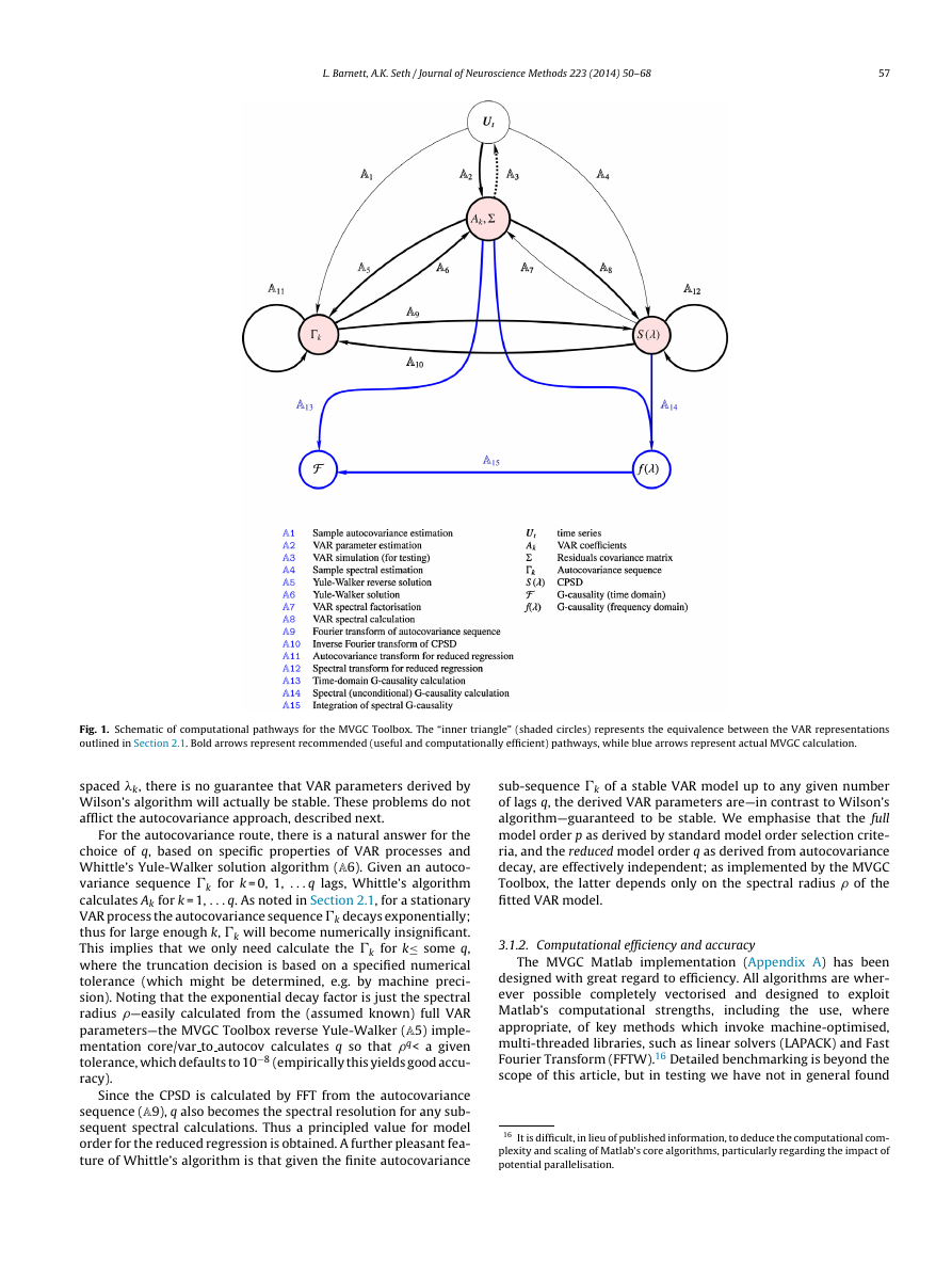A schematic of computational pathways imple- mented in the toolbox is given in Fig. 1. 3.1. Computational strategy The basic operating principle of estimation of G-causalities via the MVGC toolbox is that (after determination of a suitable model 15 In Barnett and Seth (2011) it is erroneously stated that to guarantee invariance a ﬁlter need only be causal—i.e. not contain a pure lag. In fact full invertibility (min- imum phase ﬁltering) is required to ensure that the condition (11) is not violated for the ﬁltered process. We are grateful to Victor Solo (private communication) for pointing this out. order) a VAR (1) is ﬁtted to the time series data just once (A2) and all subsequent calculations are based on the estimated model parameters ˆAk, ˆ. This approach is theoretically consistent with the fundamental assumption of G-causal estimation, that the time series data is a realisation of a stationary VAR (1). In principle, any of the equivalent VAR representations might be chosen for initial estimation—e.g. via sample autocovariance (A1 A6) or spectral estimation (A4 A7)—but empirically direct estimation (A2) proves to be the most stable, accurate and computationally efﬁcient; nonetheless the MVGC toolbox allows implementation of alternative methods. → → Having acquired the VAR model, (conditional) G-causality in the time (22) and frequency (33) domains involves estimation of VAR parameters for the reduced regressions (21) and (31) respec- tively. There is no simple algorithm (to our knowledge) to compute reduced regression VAR parameters directly from full regression parameters. Indeed, the standard approach [e.g. as implemented in Seth (2010)] is to perform the reduced regressions explicitly from the data (A2); however this leads to inaccuracies that may be particularly serious in the spectral case (see Section 2.6 and Chen et al., 2006a). Fortunately, numerical algorithms are available for obtaining reduced regression parameters from the autocovari- ance sequence (A7) via solution of the Yule-Walker equations (6), or from the CPSD (A7) via spectral factorisation (9); the autoco- variance sequence and CPSD may themselves be computed from the (full) VAR parameters by “reverse” Yule-Walker solution (A5) and straightforward spectral calculation (Fourier transform) (A8) respectively. The recommended pathway for the MVGC Toolbox is to use the autocovariance sequence. This is on the grounds that, as revealed by empirical testing over a broad range of VAR parameters, system size and model orders, Whittle’s algorithm (A8) (Whittle, 1963) for Yule-Walker solution is faster, more stable and more accurate than Wilson’s spectral factorisation algorithm (A7) (Wilson, 1972); it also has additional useful properties (see below). The toolbox thus uses the autocovariance sequence as the dominant representation for all G-causality routines (A13, A14) although, again, the alternative spectral pathways may be imple- mented if desired. Note that a useful “reality check” for the accuracy of G-causality computations is that time-domain causalities should integrate with reasonable accuracy to their spectral counterparts (34) (A15). 3.1.1. Reduced model order, spectral resolution and autocovariance lags As noted previously (Section 2.4), even if the model order for the full regression (20) is ﬁnite (and in practice a ﬁnite full model order will, of course, need to be selected), the model order for the reduced regressions (21) and (31) will be in theory inﬁnite. If, as described above, reduced VAR parameters are calculated from the autocovariance sequence (or CPSD) how do we choose a suitable ﬁnite model order? First, we note that spectral factorisation (9) speciﬁes the transfer function H() at frequencies for which the CPSD S() is speciﬁed. Now the VAR coefﬁcients Ak are calculated by matrix inversion of the transfer function followed by Fourier transform. Since the Fast Fourier Transform (FFT) (Cooley and Tukey, 1965) will be used, this implies that to calculate VAR coefﬁcients from the CPSD, the CPSD must be speciﬁed at some set of frequencies 1, . . . q evenly spaced on [0, f], where f is the sampling frequency—indeed, Wilson’s algo- rithm (A7) assumes this, and approximates the H(k) accordingly. Then the Ak will naturally be derived for k = 1, . . ., q; i.e. the spec- tral resolution q will, effectively, be the model order for the reduced regression. Unfortunately, for the spectral factorisation approach there is no obvious way to choose q. Furthermore (in contrast to Whittle’s algorithm – see below), given a CPSD S() for a stable VAR process evaluated, for a given spectral resolution q at evenly

L. Barnett, A.K. Seth / Journal of Neuroscience Methods 223 (2014) 50– 68 57 Fig. 1. Schematic of computational pathways for the MVGC Toolbox. The “inner triangle” (shaded circles) represents the equivalence between the VAR representations outlined in Section 2.1. Bold arrows represent recommended (useful and computationally efﬁcient) pathways, while blue arrows represent actual MVGC calculation. spaced k, there is no guarantee that VAR parameters derived by Wilson’s algorithm will actually be stable. These problems do not afﬂict the autocovariance approach, described next. For the autocovariance route, there is a natural answer for the choice of q, based on speciﬁc properties of VAR processes and Whittle’s Yule-Walker solution algorithm (A6). Given an autoco- variance sequence k for k = 0, 1, . . . q lags, Whittle’s algorithm calculates Ak for k = 1, . . . q. As noted in Section 2.1, for a stationary VAR process the autocovariance sequence k decays exponentially; thus for large enough k, k will become numerically insigniﬁcant. This implies that we only need calculate the k for k≤ some q, where the truncation decision is based on a speciﬁed numerical tolerance (which might be determined, e.g. by machine preci- sion). Noting that the exponential decay factor is just the spectral radius —easily calculated from the (assumed known) full VAR parameters—the MVGC Toolbox reverse Yule-Walker (A5) imple- mentation core/var to autocov calculates q so that q< a given tolerance, which defaults to 10−8 (empirically this yields good accu- racy). Since the CPSD is calculated by FFT from the autocovariance sequence (A9), q also becomes the spectral resolution for any sub- sequent spectral calculations. Thus a principled value for model order for the reduced regression is obtained. A further pleasant fea- ture of Whittle’s algorithm is that given the ﬁnite autocovariance sub-sequence k of a stable VAR model up to any given number of lags q, the derived VAR parameters are—in contrast to Wilson’s algorithm—guaranteed to be stable. We emphasise that the full model order p as derived by standard model order selection crite- ria, and the reduced model order q as derived from autocovariance decay, are effectively independent; as implemented by the MVGC Toolbox, the latter depends only on the spectral radius of the ﬁtted VAR model. 3.1.2. Computational efﬁciency and accuracy The MVGC Matlab implementation (Appendix A) has been designed with great regard to efﬁciency. All algorithms are wher- ever possible completely vectorised and designed to exploit Matlab’s computational strengths, the use, where appropriate, of key methods which invoke machine-optimised, multi-threaded libraries, such as linear solvers (LAPACK) and Fast Fourier Transform (FFTW).16 Detailed benchmarking is beyond the scope of this article, but in testing we have not in general found including 16 It is difﬁcult, in lieu of published information, to deduce the computational com- plexity and scaling of Matlab’s core algorithms, particularly regarding the impact of potential parallelisation.

资料库

格兰杰因果分析工具箱介绍（MVGC）.pdf

相关推荐

人工智能

热门标签

最新资料