Wave-front estimation from wave-front slope measurements
W. H. Southwell
Rockwell International Corporation, Rocketdyne Division, Canoga Park, California 91304
(Received 28 August 1979; revised 21 February 1980)
The problem of wave-front estimation from wave-front slope measurements has been examined
from a least-squares curve fitting model point of view. It is shown that the slope measurement
sampling geometry influences the model selection for the phase estimation. Successive over-relax-
ation (SOR) is employed to numerically solve the exact zonal phase estimation problem. A new zonal
phase gradient model is introduced and its error propagator, which relates the mean-square wave-
front error to the noisy slope measurements, has been compared with two previously used models. A
technique for the rapid extraction of phase aperture functions is presented. Error propagation prop-
erties for modal estimation are evaluated and compared with zonal estimation results.
INTRODUCTION
In this paper we consider the problem of estimating wave-
front phase from a set of discrete phase slope measurements.
This reconstruction process is necessary to obtain phase
profile estimates from certain types of sensors, such as a
shearing interferometer or a Hartmann sensor. It is also
necessary in image restoration using the Knox-Thompson'
speckle imaging technique.
A variety of approaches have been proposed to accomplish
this phase reconstruction. Basically, each estimation ap-
proach may be categorized as being either zonal or modal
depending on whether the estimate is a phase value in a local
zone or a coefficient of an aperture function. In either case,
least-squares estimation is used for the phase reconstruc-
tion.
Differences in the methods can be distinguished by the
different models used to "fit" the local slope measure-
ments.
Some important considerations in selecting a model are (i)
compatibility; does the model fit the geometry of the slope
measurements as given by the sensor?, (ii) numerical com-
plexity; are there convergence problems, storage, and com-
putation speed requirements?, and (iii) error propagation;
what effect does noise in the slope measurements have on the
phase estimates?
The reconstruction problem was first addressed in the lit-
erature by Rimmer,2 and since then by a number of authors. 3 4
Most of these papers use a phase difference slope model for
zonal reconstruction that is chiefly applicable to a shearing
interferometric sensor, where the x-slope measurement po-
sitions are not coincident with the y-slope measurement po-
sitions. With some approximations, Hudgin3 calculated the
noise propagator for this model. Using a model that assumed
coincident x- and y-slope measurements and some approxi-
mations, Fried4 also calculated the noise propagation pa-
rameter. Recently, Herrmann 8 constructed an exact solution
for the noise propagator for the models of both Fried and
Hudgin. Herrmann's results essentially confirmed the pre-
vious results.
In this paper we present a new phase reconstruction model
which, like that of Fried is applicable to coincident x- and
y-slope measurements (and thus suitable for Hartmann
sensors). The error propagation properties of this new model
have been shown to be superior to the models of both Hudgin
and Fried, partly because it provides a more uniform sampling
of the aperture. We also describe, and illustrate with exam-
ples, a matrix iterative technique that solves the exact least-
squares zonal reconstruction problem, is easy to implement,
and exhibits rapid convergence.
Modal estimation is also discussed. Some numerical
methods for the rapid extraction of the low-order orthogonal
modes are described. Finally, noise propagation effects using
modal estimation are compared with those using zonal esti-
mation.
ZONAL ESTIMATION
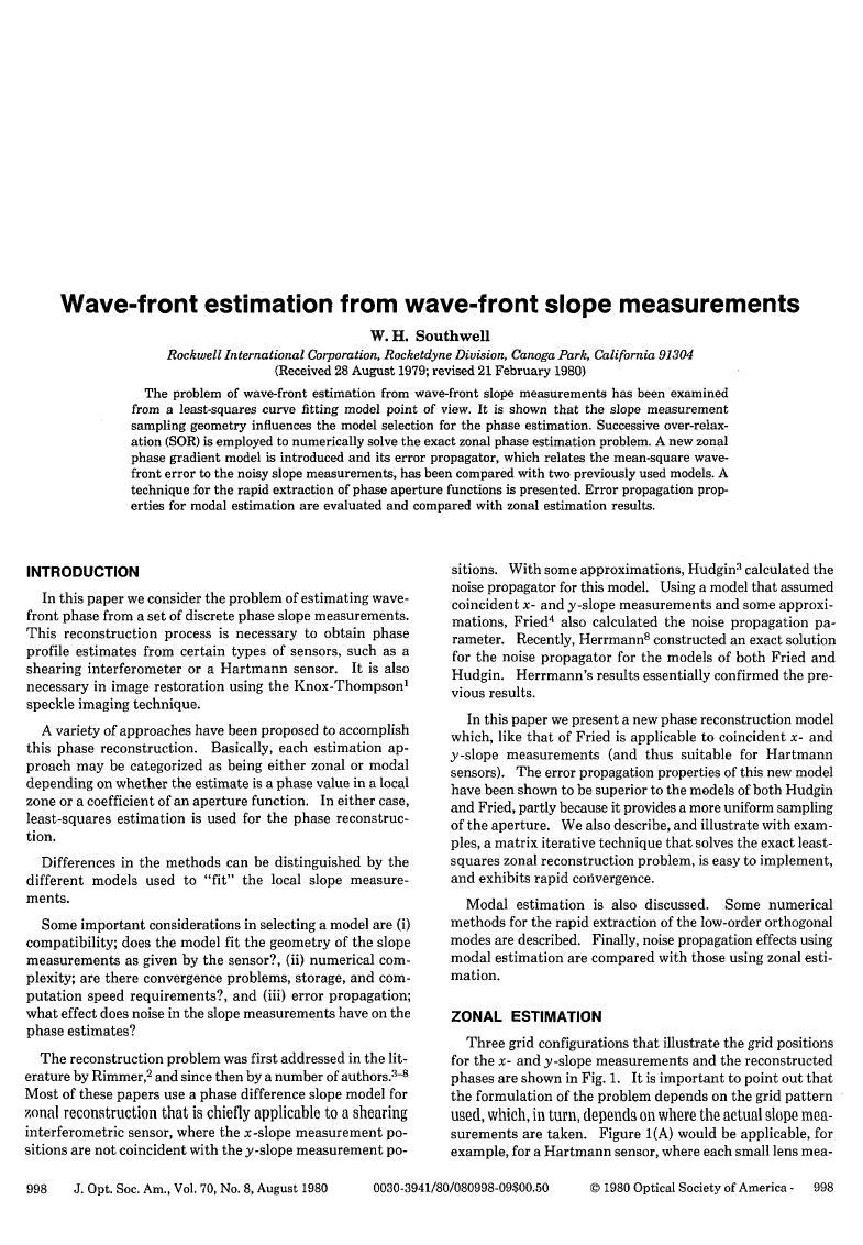
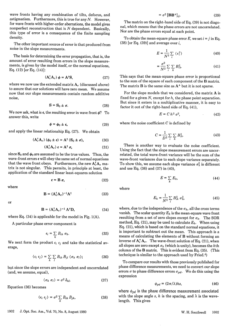
Three grid configurations that illustrate the grid positions
for the x- and y-slope measurements and the reconstructed
phases are shown in Fig. 1. It is important to point out that
the formulation of the problem depends on the grid pattern
used, which, in turn, depends on where the actual slope mea-
surements are taken. Figure 1(A) would be applicable, for
example, for a Hartmann sensor, where each small lens mea-
998
J. Opt. Soc. Am., Vol. 70, No. 8, August 1980
0030-3941/80/080998-09$00.50
(0 1980 Optical Society of America -
998
�
Syj = (bij+1- oij)/h
1J
i= 1, N
i= 1,N- 1
1
(6)
where h = DIN and D is the width of the aperture. Each
phase point represents an equal subregion of area h 2 in the
aperture. This is the least-squares model used by Hudgin.3
(We note that it is equivalent to the assumption of a bilinear
spline phase on the phase grid of Fig. 1(B). The phase is ev-
erywhere continuous, but has discontinuous slopes at the mesh
points.)
It is also interesting to note that we have derived the slope
model based on actual local slopes. But we see from Eqs. (5)
and (6) that the model is equally applicable to the assumption
that the slopes be determined by adjacent phase differ-
ences.
Now suppose our x- and y-slope measurements are given
at coincident points, as in a Hartmann plate. One possibility
is to let the phase points used in Eq. (4) be replaced by the
average of two phase values which are positioned perpendic-
ular to the slope direction by one half-step up and one half-
step down. This is the configuration shown in Fig. 1(C). This
gives the slope model used by Fried,4
Sx = [(¢0i+1j, + oi+lj+,)/ 2 - (kij +
h
,ij++)/2]
= [(0jj+1 +
±i+lj+i)/2 -(kij + 0i+ij)/2]
1]
h
(7)
(8)
For a new model appropriate for Hartmann sensor mea-
surements, we consider the grid geometry of Fig. 1(A) and
return to Eqs. (1) and (2) for a representation of the phase
between mesh points. This time we have two measurements
per interval, a slope at each end. This enables the determi-
nation of both cl and c2 in Eq. (2).
This produces the relationships
(Sj,X~,j + S,,j)
(Oi+,j -r oij)
2
(Stx+ j + SY0-
2
h
(0i'j+1 -
h
ij)
I
i = 1, N-
j= 1,N
i= 1,N
j= 1,N-1
MI
(10)
[We comment that the phase model used for data configu-
ration like Fig. 1 (A) is a biquadratic spline, whereas configu-
rations like Fig. 1(B) are based on a bilinear spline phase.
However, since we are not interpolating, but only determining
the phase at the mesh points, it does not necessarily mean that
one is more accurate in the phase estimation.]
LEAST-SQUARES SOLUTION
Having a set of measurements Sx and SY and a model for
these quantities [Eqs. (5) and (6), (7) and (8), or (9) and (10)
in terms of the adjustable parameters Iij], it is straightforward
to apply least-squares techniques. However, there are some
potential difficulties which require attention.
To formulate the least-squares problem, note that Eqs. (5)
and (6) or Eqs. (7) and (8) may be written as a single matrix
equation
S=A4,
(11)
where S is a vector containing all the slope measurements (x
(B)
I I I 1.
*,-
___
j
4 -
+ -
"
-
I
*-*9-*-
-
I
FIG. 1. Slope measurement
sampling geometry and wave-
front mesh points. The horizontal
dashes indicate positions of x-
slope sampling.
The vertical
dashes are the y-slope sampling
positions. The dots are the esti-
mated phase points. Configura-
tion B has been considered pre-
viously by Hudgin and configura-
tion C by Fried.
sures both the x andy slopes at the same point. Figure 1(B)
could be applicable, for example, in a shearing interferometer
where the beam is first divided in order to apply, separately,
the x and y shears. Figure 1(C) shows coincident x and y
slopes, but with a displaced phase grid.
The problem is to least-squares-fit the slope measurement
data to some function or model of the phase given at its grid
points. Consider first the data configuration given in Fig.
In that configuration there are N2 phase points and
1(B).
2N(N-1) slope measurement points. Let us assume that the
phase dependence between grid points in the x direction is
represented by the polynomial
The slope is
t1=Co +
clx
2
.
Sx = c1 + 2c 2x.
(1)
(2)
But since we have only one slope measurement, which is given
at the midpoint of the interval, we can only determine c 1. The
constant c0 is the value of the phase at the left side of the in-
terval. Thus, all that the data can support is a linear phase
model,
q5= + ST x.
(3)
The phase at the right of the interval (x =h) is ki+ . Applying
this boundary fact leads to the slope model,
S-T = (0i+1 - ,i)lh
i = 1, N- 1,
(4)
where N is the number of phase sample points in the x direc-
tion. Generalizing to all rows and to the y direction, we ob-
tain,
= - 1N - 1
j1, N
()
999
J. Opt. Soc. Am., Vol. 70, No. 8, August 1980
W. H. Southwell
999
�
slopes first) and 4 is a vector of length N2 containing all the
unknown phase values. The size of the rectangular matrix
A is N2 by the number of slope measurements; however, it is
very sparse. Multiplying Eq. (14) from the left by At (A
transpose), we obtain the normal equations
(AtA)o = AtS,
(12)
which are a set of N 2 linear equations in N2 unknowns 4jk.
The standard least-squares solution is obtained by multi-
plying the right-hand side of Eq. (12) by the inverse of the
square matrix AtA.
However, the standard least-squares solution cannot be
used because AtA is singular. This is a consequence of the
fact that any constant wave front added to the correct wave
front also satisfies the models. This does not mean that Eq.
(12) cannot be solved for a meaningful solution. But it does
mean we cannot use the standard matrix inversion tech-
nique.
Herrmann has shown that the desired solution is the one
that has a minimum norm, which has zero mean. He shows
that using the zero-mean condition leads to an extended Ae
matrix that yields an At A, matrix that is not singular. The
matrix A, has an additional row (of all ones) and Se has an
additional element (zero). However, this procedure requires
the computer storage of a matrix the size A, which has es-
sentially 2N2 elements.
For large arrays, we can use iterative matrix methods for
solving Eq. (12). The solution obtained is unique to within
an additive constant, but it is an easy matter to subtract out
the mean. We discuss these methods below. But first, we
write the matrix equation representing Eqs. (9) and (10), the
Fig. 1(A) model,
DS = A4,
(13)
where D is a large sparse matrix that performs the adjacent
slope averaging. The corresponding normal equations are
(AtA)4) = AtDS.
(14)
MATRIX
ITERATIVE SOLUTIONS
For large arrays, we can take advantage of the sparse nature
of AtA and use matrix iterative methods for solving Eqs. (12)
and (14). If we write just the nonzero matrix element com-
ponents of Eq. (12) for Fig. 1(B) configuration, we obtain
gJ'kJjh
[bj+lk + )j-l, +
'jk+1 +
'kj,k-1I
= [SJ1k--
SJk + Si-I,k Sjk] h,
(15)
where
2
j=lorN;k=lorN
gj = 3
4
lj =1 or N; = 2to N -
= k = 1 orN; j = 2toN -1
otherwise,
(16)
and if a nonexistent matrix element is called for, then zero is
assumed. The g factors are the diagonal elements of AtA,
which are either 2, 3, or 4 according to whether its accompa-
nying phase point qpjh is on a corner, an edge, or an interior
point. Calling the right-hand side bjk, we can rewrite Eq. (15)
as
'tjk = kjk + bJhlgjk,
where opii is the nearest-neighbor phase average,
jth = [j+l,k + Oj-l,k + 4j,k+l]/gJk,
and
bib = [Syk-I - S\ + S-ik
- SJk'h,
(17)
(18)
(19)
which is a constant depending only on the slope measure-
ments.
Equation (17) forms the basis for an iterative solution. The
right-hand side of Eq. (17) is evaluated using current values
for the O's (which may initially be zero). The result becomes
the improved estimate; at the mth iteration, this becomes
Oj(hm+l) =
J(km) + biklgih-
(20)
If the left-hand side is held in a separate array until all N2
points are evaluated, then this procedure is the Jacobi method.
If, however, the left-hand side updates the wave-front array
directly, such that succeeding evaluations of the right-hand
side could use phase points that have already been updated,
then the procedure is called the Gauss-Seidel method.
Generally, the Gauss-Seidel method converges faster and is
easier to implement.
Neither of these methods, however, updates a phase point
based on the previous value at that point, since 4)jh does not
include 4)k-
By adding and subtracting 4)jk on the right-hand side of Eq.
(20) and introducing the relaxation parameter a, we have
(m +1) = (m) + . [2 ) + bjk/gjk - 0)J1 ]
(21)
This iterative technique is the successive over-relaxation
(SOR) method. Convergence is achieved when the quantity
in brackets on the right-hand side becomes small. The SOR
method generally promises improvement in convergence;
however, it is necessary to determine the value of the relaxa-
tion parameter w which maximizes the rate of convergence.
Fortunately, AtA for the phase reconstruction problem
belongs to a class of matrices for which the optimal value of
w is known.9 The result is
2
W 1 + sin[7r/(N + 1)]
(22)
The results of a numerical comparison of the three matrix
iteration methods discussed above are tabulated in Table I.
The slope measurements were generated from the analytical
derivatives of a simulated wave front, which in this example
contained astigmatism. The rms wave-front reconstruction
error was calculated by comparing the wave front recon-
structed from the slopes with the simulated wave front. The
Jacobi method converged but left a small residual error in this
example, although it generally gives the correct answer. The
Gauss-Seidel method converged in approximately N2 itera-
tions, whereas the SOR method converged in approximately
2N iterations.
(An analysis of the convergence rates indicates
that for large N, SOR will converge 2N/7r fewer iterations than
the Gauss-Seidel method.)
Hudgin 3 formulates the wave-front reconstruction problem
in such a way that edge effects are ignored. They deal with
Eq. (15) where all the gjk = 4, which treats all phase points as
1000
J. Opt. Soc. Am., Vol. 70, No. 8, August 1980
W. H. Southwell
1000
�
rms wave-front reconstruction error in waves as a function of
TABLE I.
the number of iterations for three different iterative methods. The sampled
2 )/a2
wave front contained astigmatism of the form W = 2.3717 (X2
+ 6xyla2 over a square aperture of area 4a 2.
-y
N
4
8
16
Number of
iterations
Jacobi
Gauss-Seidel
SOR
2
4
8
16
32
64
2
4
8
16
32
64
128
256
2
4
8
16
32
64
128
256
512
1024
0.487
0.176
0.126
0.125
0.125
0.125
1.638
1.288
0.823
0.350
0.067
0.014
0.013
0.013
2.068
1.947
1.744
1.422
0.969
0.467
0.113
0.007
0.002
0.002
0.504
0.255
0.043
8)x 10-4
3 X 10⁻⁷
0
1.389
0.936
0.454
0.151
0.034
0.002
4)x 10-6
0
1.963
1.763
1.446
0.996
0.492
0.135
0.022
0.001
6 x 10⁻⁶
0
0.620
0.249
2 x 10⁻⁴
0
0
0
1.062
0.664
0.319
0.022
6 X 10⁻⁵
0
0
0
1.563
1.159
0.716
0.344
0.046
5x 10⁻⁴
0
0
0
0
being in the interior of the aperture. Such an assumption can
lead to large wave-front reconstruction errors. Table II shows
the wave-front reconstruction results using the recursive al-
gorithm of Hudgin on the same slope data used in Table I.
The large errors indicate that the simulated wave front was
not reconstructed. This means that edge effects are impor-
tant-even for N = 16, where nearly one-fourth of the phase
points lie on the aperture edge.
Frost et al.7 also neglect edge effects in order to utilize a
fast-Fourier-transform solution method. The results of their
numerical examples appear to be quite good; however, they
used a large phase grid, N = 256.
For practical wave-front sensors, where N will probably be
less than 35, the aperture boundary or edge effects are im-
portant. To make this point more explicit, we used the re-
cursive algorithm of Hudgin on a simulated wave front with
defocus W = 1.732 [2(x 2 + y 2) - 1]. Using an N = 4 grid, the
correct wave front is
/2.17
1 0.43
0.43
2.17
0.43
-1.30
-1.30
0.43
0.43 2.17\
-1.30 0.43
-1.30 0.43
0.43 2.17
(23)
The exact analytical derivatives were used to generate the
slope data at the midpoints between sample points. The re-
constructed wave front, using the recursive formula of Hudgin,
gave the following result (after applying an unimportant
constant offset of 1.588):
1001
J. Opt. Soc. Am., Vol. 70, No. 8, August 1980
2.17
1 1.01
1.01
2.17
1.01
-0.72
-0.72
1.01
1.01 2.17\
1.01
-0.72
-0.72
1.01 )
1.01 2.17
(24)
The rms wave-front reconstruction error was 0.25 waves.
We next write the nonzero matrix element components of
Eq. (14), Fig. 1(A) configuration:
gjkIjk -
[Oj+l,k +
'j-lk
+ kj,k+l + Oj,k-1]
1
= -
2'
[Sjyh+l -Sjyk-1 ± Sjx+l,k -S1_1,k] h,
(25)
where
2
j=lorN;k=lorN
gjk =
3 kl1orN;j-2toN-1
4
otherwise,
(26)
and if a nonexistent phase element is called for, then zero is
assumed, and if a nonexistent slope element is called for, then
the negative of the adjacent slope is assumed. The only dif-
ference between this equation and Eq. (15) is in the formation
of the right-hand side of Eq. (25), which is only a manipulation
of the data. Consequently, the same SOR technique, Eq. (21),
may be applied, except that bik is now the right-hand side of
Eq. (25).
ZONAL ESTIMATION ERROR
There are two important sources of error in the recon-
struction process. One is the algorithm accuracy. That is,
how well does the least-squares process reconstruct a phase
of arbitrary shape? The answer, of course, depends on the
shape of the wave front being measured. For example, nu-
merical experimentation indicates that the zonal recon-
struction models discussed here will perfectly reconstruct
TABLE II. Wave-front reconstruction results using the recursive formula
of Hudgin (which neglects edge effects). Shown here is the rms wave-front
reconstruction error in waves from slope data sampled from a wave front
containing astigmatism of the form W = 2.3717(x 2 - y2)/a 2 + 6xy/a2 over
a square aperture of area 4a 2 .
In each case the recursive algorithm quickly
converged, but did not reproduce the sampled wave front.
Number of
iterations
rms error
2
4
8
16
2
4
8
16
2
4
8
16
1.106
1.158
1.160
1.159
1.624
1.602
1.625
1.624
1.944
1.905
1.897
1.908
N
4
8
16
W. H. Southwell
1001
�
wave fronts having any combination of tilts, defocus, and
astigmatism. Furthermore, this is true for any N. However,
for wave fronts with higher-order aberrations, the model gives
nonperfect reconstruction that is N dependent. Basically,
this type of error is a consequence of the finite sampling
density.
The other important source of error is that produced from
noise in the slope measurements.
The basis for determining the error propagation, that is, the
amount of error resulting from errors in the slope measure-
ments, is given by the model itself, or the normal equations,
Eq. (12) [or Eq. (14)]:
(AtAe) O = AtS,
(27)
where we now use the extended matrix Ae (discussed above)
to assure that our solutions will have zero mean. We assume
now that our slope measurements contain random additive
noise,
(28)
We now ask, what is e, the resulting error in wave front O? To
answer this, write
S = So + a.
and apply the linear relationship Eq. (27). We obtain
0 = t0o
:
,
(AlA,) (Oo + e) = At (So ± a),
(AtAe) e = At or,
(29)
(30)
(31)
since So and 00 are assumed to be the true values. Thus, the
wave-front errors e will obey the same set of normal equations
that the wave front obeys. Furthermore, the new AtAe ma-
trix is not singular. This permits, in principle at least, the
application of the standard linear least-squares solution
where
e= B a,
B = (AtAe)-At
B = (AtAeA)-
1 AtD,
where Eq. (34) is applicable for the model in Fig. 1(A).
A particular phase error component is
e= E Bik ak.
k
(32)
(33)
(34)
(35)
We next form the product Ej ej and take the statistical av-
erage,
(ei ej) = A E Bih B1 l (a, al);
k
I
(36)
bvt since the slope errors are independent and uncorrelated
(and, we assume, equal),
((k CO) = a2 6k1.
Equation (36) becomes
(Ei EJ) = a2EZBikBik,
k
(37)
(38)
2
[BB+]iLJ
= U
(39)
The matrix on the right-hand side of Eq. (39) is not diago-
nal, which means that the phase errors are not uncorrelated.
Nor are the phase errors equal at each point.
To obtain the mean-square phase error E, we set i = j in Eq.
(38) [or Eq. (39)] and average over i,
E =
E_ (BE2)
= N2 E_ E B'k
(40)
(41)
This says that the mean-square phase error is proportional
to the sum of the square of each component of the B matrix.
The matrix B is the same size as A+ but it is not sparse.
For the slope models that we considered, the matrix A is
fixed for a given N, except for h, the phase point separation.
But since it enters in a multiplicative manner, it is easy to
factor it out of the right-hand side of Eq. (41),
E= Ch2 U2,
where the noise coefficient C is defined by
C = D2 L L Bik
(42)
(43)
There is another way to evaluate the noise coefficient.
Using the fact that the slope measurement errors are uncor-
related, the total wave-front variance will be the sum of the
wave-front variances due to each slope variance separately.
To show this, we assume each slope variance Sk is different
and use Eq. (36) and (37) in (40),
where
E = Z Ek,
k
Eh = I L, B2 a2
(44)
(45)
where, due to the independence of the ak, all the cross terms
vanish. The scalar quantity Ek is the mean-square wave front
resulting from a set of zero slopes except for Uk. The SOR
method, Eq. (21), may be used to calculate Ek. When using
Eq. (21), which is based on the standard normal equations, it
is important to subtract out the mean. This approach is a
means of calculating the elements of B without forming an
inverse of A'Ae. The wave-front solution of Eq. (21), when
all slopes are zero except 0Uk (which is unity), becomes the kth
column of the B matrix. This is evident from Eq. (35). (This
technique is similar to the approach used by Fried.4 )
To compare our results with those previously published for
phase difference measurements, we need to convert our slope
errors a to phase difference errors 0Ipd- We do this using the
expression
Opd = (2r/X)hs,
(46)
where ()pd is the phase difference measurement associated
with the slope angle s, h is the spacing, and X is the wave-
length. This gives
1002
J. Opt. Soc. Am., Vol. 70, No. 8, August 1980
W. H. Southwell
1002
�
1.6-
1.2-
0.81
0.4
C
B
A
_1
I I
2I
I
20
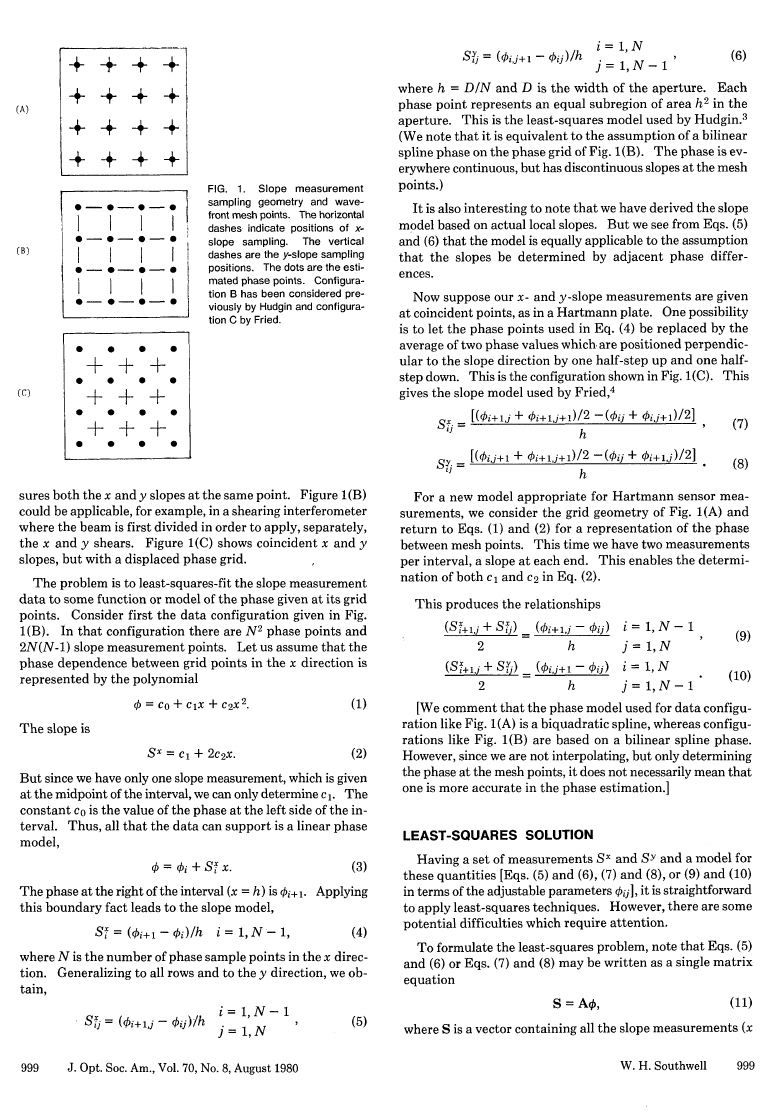
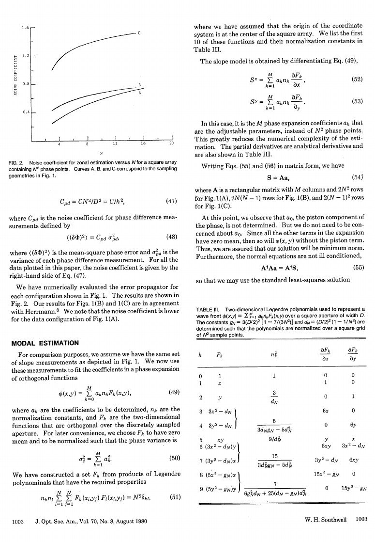
FIG. 2. Noise coefficient for zonal estimation versus N for a square array
containing N2 phase points. Curves A, B, and C correspond to the sampling
geometries in Fig. 1.
N
Cpd = CN2/D 2
= C/h2 ,
(47)
where Cpd is the noise coefficient for phase difference mea-
surements defined by
r2
=
)CPd pd,
(48)
where ((634)2) is the mean-square phase error and apd is the
variance of each phase difference measurement. For all the
data plotted in this paper, the noise coefficient is given by the
right-hand side of Eq. (47).
We have numerically evaluated the error propagator for
each configuration shown in Fig. 1. The results are shown in
Fig. 2. Our results for Figs. 1(B) and 1(C) are in agreement
with Herrmann. 8 We note that the noise coefficient is lower
for the data configuration of Fig. 1(A).
MODAL ESTIMATION
For comparison purposes, we assume we have the same set
of slope measurements as depicted in Fig. 1. We now use
these measurements to fit the coefficients in a phase expansion
of orthogonal functions
O(x,y) = E aknkFk(X,y),
M
k=O
(49)
where ak are the coefficients to be determined, nk are the
normalization constants, and Fk are the two-dimensional
functions that are orthogonal over the discretely sampled
aperture. For later convenience, we choose Fk to have zero
mean and to be normalized such that the phase variance is
co
M
2
2=
E_ ak.
k=1
(50)
7 (3ye-1dN)X
7 (3y2.Nd2)x)-
15
d
We have constructed a set Fk from products of Legendre
polynominals that have the required properties
8 (5X 2 -gN)x
nkni E
E Fk (xivyj) Ft (xi~yj) = N
N N.
j=1 j=1
41l,
(51)
9 (5y 2 -gN)y) 6gNdN + 25(dN-gN)dN
0
15y 2 -gN
1003
J. Opt. Soc. Am., Vol. 70, No. 8, August 1980
W. H. Southwell
1003
where we have assumed that the origin of the coordinate
system is at the center of the square array. We list the first
10 of these functions and their normalization constants in
Table III.
The slope model is obtained by differentiating Eq. (49),
M
SX = E aknk-
k=1
ax
k
M
SY= E akank
k=1
ZFk
CY
(52)
(53)
In this case, it is the M phase expansion coefficients ak that
are the adjustable parameters, instead of N 2 phase points.
This greatly reduces the numerical complexity of the esti-
mation. The partial derivatives are analytical derivatives and
are also shown in Table III.
Writing Eqs. (55) and (56) in matrix form, we have
S = Aa,
(543
where A is a rectangular matrix with M columns and 2N 2 rows
for Fig. 1(A), 2N(N - 1) rows for Fig. 1(B), and 2(N - 1)2 rows
for Fig. 1(C).
At this point, we observe that ao, the piston component of
the phase, is not determined. But we do not need to be con-
cerned about ao. Since all the other terms in the expansion
have zero mean, then so will 0(x, y) without the piston term.
Thus, we are assured that our solution will be minimum norm.
Furthermore, the normal equations are not ill conditioned,
AtAa = AtS,
(55)
so that we may use the standard least-squares solution
TABLE Ill. Two-dimensional Legendre polynomials used to represent a
wave front b(xy) = M 1 aknkFk(xy) over a square aperture of width D.
3(D/2)2 [1- 7/(3N2)] and dN = (D/2) 2 (1 - 1/N2) are
The constants gN
determined such that the polynomials are normalized over a square grid
of /N2 sample points.
k
0
1
2
Fk
1
x
Y
3
3x 2 -dNp
4 3y 2 -dN J
5
6 (3X2 - dN)y
xy
nk
1
3
3
dN
5
3dNgN-5dN
9NdN
Fk
Fk
0
1
0
6x
0
0
0
1
0
6y
y
6xy
x
3x 2 - dN
3y2 -dN
6xy
15x2 -gN
0
�
a = (AtA)-'AtS,
(56)
where AtA is an M by M symmetric matrix, and AtS is a
vector of length M whose components are weighted sums (or
moments) over the slope data.
From an inspection of the partial derivatives listed in Table
III, we note that many of them turn out to be other Fk func-
tions. Thus, those are orthogonal. Fitting data directly to
an orthogonal set has the advantage that each may be deter-
mined independently by a weighted sum over the data. In
terms of Eq. (56), this results in a diagonal MA matrix. In-
version of a diagonal matrix requires no lengthy numerical
procedure. The inverse is also diagonal with the diagonal
elements being the reciprocals of corresponding elements.
As an example, suppose we wish to extract all modes up to
and including astigmatism, M = 5. For N = 4 this gives
AtA =
/1.2
0
°
0
0
0
51.2
0
0
0
0
0
32.0
0
0
0
0
0
32.0
0
0
0
0
0
102. 4)
[AtA-1 =
0.0195
0
0
0
0
o
0.0195
0
0
0
0
0
0.0031
0
0
0
0
0
0.0031
J.
(58)
0
0.0098/
Furthermore, we note that these matrix elements are not data
dependent. They depend only on the sensor geometry such
as N. This means they may be fixed, predetermined numbers
in Eq. (56). The mode extraction then reduces to a weighted
sum over the slope data. In some cases, this sum extends only
x- or y-slope data.
Suppose we wish to extract all nine modes shown in Table
III. In this case, we note that the derivative of F 8 is not or-
thogonal to the derivative of F1 . This leads to an AtA matrix
that is no longer diagonal. Fortunately, this is not a serious
difficulty. It does not mean we lose the fast mode extraction
discussed above for the other modes.
In this case the only
off-diagonal elements that appear are 1 and 8, and 2 and 9.
For the unaffected modes, the inverse is still the reciprocal of
the diagonal element. For the modes that are coupled, the
inverse is just the inverse of the 2 X 2 submatrix. Thus, the
inverse of AtA is as sparse as AtA. To demonstrate this, we
write these matrixes for N = 4,
51.2
0
0
0
0
0
0,
145.1
0
51.2
0
0
0
0
0
0
0
145.1
0
0.0258
0
0
320.
0
0
0
0
0
0
0
0
0
0
0
0
0
0
0.0031-2
0
0
0
0
0
0
0
-0.00211
AtA =
0.0258
0
0
0
0
0
0
-0.00211
(AtA)-l =
l
0
0
0
0
102.4
0
0
0
0
0
0
0
320.
0
0
0
0
0
0
0
0
0.003 12
0
0
0
0
0
0
0
0
0
0.00977
0
0
0
0
i
0
0
0
0
0
371.2
0
0
0
0
0
0
0
0
0
371.2
0
0
0
0
0
0
0
0.00269
145.1
0
0
0
0
0
0
1691.
0
0
145.1
0
0
0
0
0
0
1691.
0
0
0
0
0
0
-0.00211
0
0
0
0
0
0
0
0.00078
0
-0.00211
0
0
0
0
0
0
0.00078
0
0
0
0.00269
0
0
(59)
(60)
(62)
Thus, mode extraction is still numerically fast. For uncoupled
modes, they are determined by independent weighted sums
of the slope data. For coupled modes, it is a linear combina-
tion of the weighted sums for those modes.
MODAL ESTIMATION ERROR
In order to compare the noise propagation properties of
modal reconstruction, we next determine the phase error Ei
at the discrete grid points, as we did above for the zonal re-
construction. Using Eq. (32) and
a = a
(61)
where a is the induced random error in the modal coefficients
due to the slope measurement noise, we have, from Eq.
(49),
cta,
Ei = Ec aInIF1 (xi,yi).
l
Note that ei automatically has zero mean due to our definition
of the F1 functions. Thus, the mean-square phase recon-
struction error E is
E = N2 E
=
(63)
where we have used the orthogonality of the F1 functions. We
now use Eq. (56) with Eqs. (28) and (61) to obtain al
=(a2)
cal = E [(A+A)-'A+J]1 joj.
j
This gives from Eq. (63)
(64)
1004
J. Opt. Soc. Am., Vol. 70, No. 8, August 1980
W. H. Southwell
1004
�
0.8
-
0.6
-
0.4
-
B
0.2
5
10
15
20
25
30
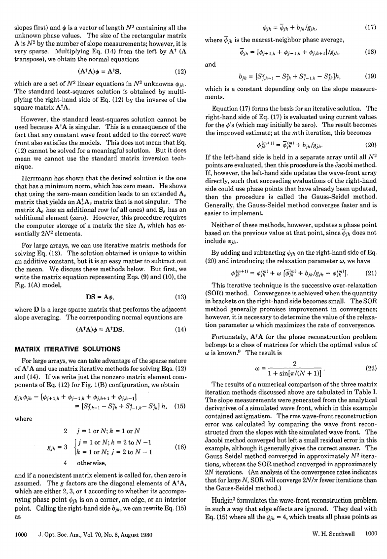
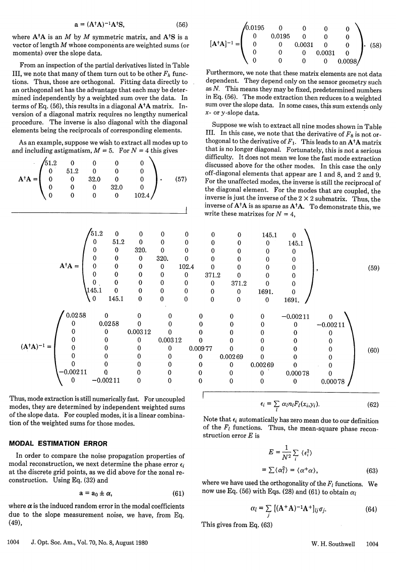
FIG. 3. Noise coefficient for
modal estimation versus N for a
square array containing N2 phase
points. Curves A, B, and C cor-
respond to the sampling geome-
tries in Fig. 1.
E = E_ E EZ [(A+A)- 1A+]ij [A+(A+A)- 1]kI (ajgfk).
I
j k
Ensemble averaging of the slope errors gives
(i ap) )=
2 5jk,
(65)
(66)
where we assume the errors are equal and uncorrelated.
Applying Eq. (66) to Eq. (65), we have
E= E E [(AtA)-lAt]j [A(AtA)-t~1ji2
=L[(AtA)-1AtA(AtA)-1J11 52
= a2
(AtA)ul = 2 tr(AtA)-.
(67)
Thus, the mean-square phase error is proportional to the
trace of (AtA)-', which is the sum of the diagonal ele-
ments.
Using our previous definition for C, Eqs. (42) and (47), the
error propagation parameter, we have
CMR = -
tr(AtA)-1 , modal reconstruction,
(68)
where h is the distance between sample points.
Equations (58) and (60) give us the breakdown by modes
of CMR for N = 4, where we can examine the diagonal elements
term by term. The data geometry used was as shown in Fig.
1(A).
We evaluated CMR for all data configurations shown in Fig.
1 for several values of N. The results for nine modes are
shown in Fig. 3. For small N, like the zonal reconstruction,
there is significant difference between the three cases.
The difference may be accounted for by two factors. The
first is that the number of data points differs in each case. For
Fig. 1(A) we have 2N2 slopes, for 1(B) there are 2N(N - 1),
and for 1(C) there are 2(N - 1)2. The second factor is their
location. We note from Fig. 1(C) that we are reconstructing
the phase outside the slope sampling region. Phase recon-
struction in this region is, like extrapolation, more uncertain.
Cubalchini 10 has also observed that the error propagation
depends on the slope geometry (for modal estimation).
DISCUSSION AND CONCLUSIONS
The above explanation may also account for the difference
between the zonal reconstruction models of Hudgin and Fried
previously reported (and shown as curves B and C in Fig. 2).
As might be expected, these differences become smaller as N
increases for modal estimation. But for zonal estimation, we
note that the differences between the Fig. 1(A) and 2(A)
geometries become smaller, but the large gap to Fig. 1(C) ge-
ometry (and model) appears to persist even at large N.
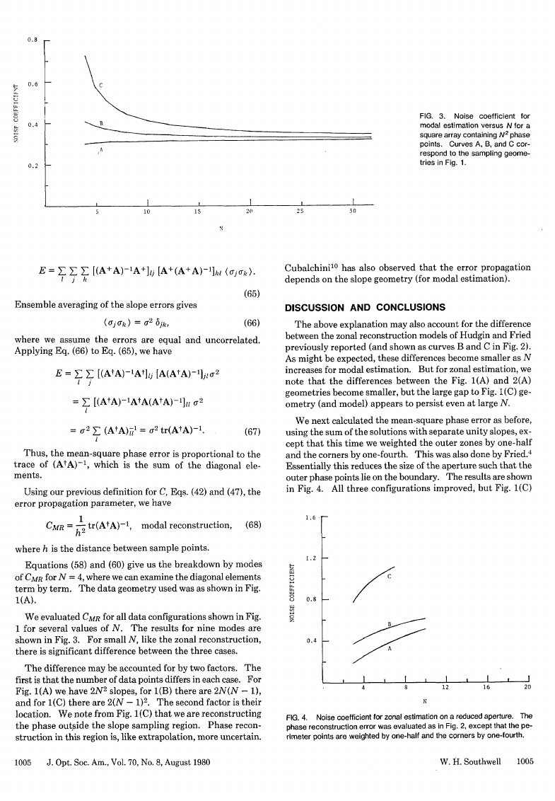
We next calculated the mean-square phase error as before,
using the sum of the solutions with separate unity slopes, ex-
cept that this time we weighted the outer zones by one-half
and the corners by one-fourth. This was also done by Fried.4
Essentially this reduces the size of the aperture such that the
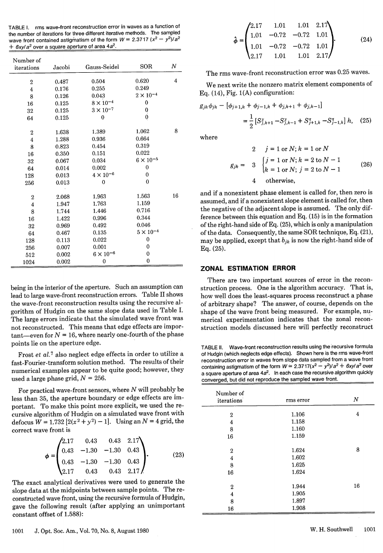
outer phase points lie on the boundary. The results are shown
in Fig. 4. All three configurations improved, but Fig. 1(C)
1.6 r
1.2 F-
4-z
0. 8 F-
0.4
C
__B~
A
I /
4
8
12
N
I
I
16
I
I
20
FIG. 4. Noise coefficient for zonal estimation on a reduced aperture. The
phase reconstruction error was evaluated as in Fig. 2, except that the pe-
rimeter points are weighted by one-half and the corners by one-fourth.
1005
J. Opt. Soc. Am., Vol. 70, No. 8, August 1980
W. 14. Southwell
1005
�


 2023年江西萍乡中考道德与法治真题及答案.doc
 2012年重庆南川中考生物真题及答案.doc
 2013年江西师范大学地理学综合及文艺理论基础考研真题.doc
 2020年四川甘孜小升初语文真题及答案I卷.doc
 2020年注册岩土工程师专业基础考试真题及答案.doc
 2023-2024学年福建省厦门市九年级上学期数学月考试题及答案.doc
 2021-2022学年辽宁省沈阳市大东区九年级上学期语文期末试题及答案.doc
 2022-2023学年北京东城区初三第一学期物理期末试卷及答案.doc
 2018上半年江西教师资格初中地理学科知识与教学能力真题及答案.doc
 2012年河北国家公务员申论考试真题及答案-省级.doc
 2020-2021学年江苏省扬州市江都区邵樊片九年级上学期数学第一次质量检测试题及答案.doc
 2022下半年黑龙江教师资格证中学综合素质真题及答案.doc