A User Manual for the Fisher Information Matrix
Jet Propulsion Laboratory, California Institute of Technology, Pasadena, CA 91109
(Dated: Feb 9 2007)
Michele Vallisneri
The Fisher-matrix formalism is used routinely in the literature on gravitational-wave detection
to characterize the parameter-estimation performance of gravitational-wave measurements, given
parametrized models of the waveforms, and assuming detector noise of known colored Gaussian
distribution. Unfortunately, the Fisher matrix can be a poor predictor of the amount of information
obtained from typical observations, especially for waveforms with several parameters and relatively
low expected signal-to-noise ratios, or for waveforms depending weakly on one or more parameters,
when their priors are not taken into proper consideration.
I discuss these pitfalls and describe
practical recipes to recognize them and cope with them.
Specifically, I answer the following questions: (i) What is the significance of (quasi-)singular
Fisher matrices, and how do we deal with them? (ii) When is it necessary to take into account
prior probability distributions for the source parameters? (iii) When is the signal-to-noise ratio high
enough to believe the Fisher-matrix result?
PACS numbers: 04.80.Nn, 95.55.Ym, 02.50.Tt
I.
INTRODUCTION
Over the last two decades, the prevailing attitude in the gravitational-wave (GW) source-modeling community
has been one of pre-data positioning:
in the absence of confirmed detections, the emphasis has been on exploring
which astrophysical systems, and which of their properties, would become accessible to GW observations with the
sensitivities afforded by planned (or desired) future experiments, with the purpose of committing theoretical effort to
the most promising sources, and of directing public advocacy to the most promising detectors. In this positioning and
in this exploration, the expected accuracy of GW source parameters, as determined from the signals to be observed,
is often employed as a proxy for the amount of physical information that can be gained from detection campaigns.
However, predicting the parameter-estimation performance of future observations is a complex matter, even with the
benefit of accurate theoretical descriptions of the expected waveforms and of faithful characterizations of the noise and
response of detectors; and in practice, the typical source modeler has had much less to go with. The main problem
is that there are few analytical tools that can be applied generally to the problem, before resorting to relatively
cumbersome numerical simulations that involve multiple explicit realizations of signal-plus-noise datasets.
In the source-modeling community, the analytical tool of choice has been the Fisher information matrix Fij[h] =
(hi, hj): here hi(t) is the derivative of the gravitational waveform h(t) of interest with respect to the i-th source
parameter θi, and “(·,·)” is a signal product weighted by the expected power spectral density of detector noise, as
−1
described in Sec. II B. Now, it is usually claimed that the inverse Fisher matrix F
ij [h0] represents the covariance
matrix of parameter errors in the parameter-estimation problem for the true signal h0. This statement can be
interpreted in three slightly different ways (all correct), which we examine in detail in Sec. II, and preview here:
1. The inverse Fisher matrix F
−1
ij [h0] is a lower bound (generally known as the Cram´er–Rao bound) for the error
covariance of any unbiased estimator of the true source parameters. Thus, it is a frequentist error (see Sec.
II A): for any experiment characterized by the true signal h0 and a certain realization n of detector noise, the
−1
parameter estimator ˆθ is a single-valued function of the total detector output s = n + h0, and F
ij [h0] is a
lower bound on the covariance (i.e., the fluctuations) of ˆθ in an imaginary infinite sequence of experiments with
different realizations of noise. The Cram´er–Rao bound is discussed in Sec. II C.
2. The inverse Fisher matrix F
−1
ij [h0] is the frequentist error covariance for the maximum-likelihood (ML) parameter
estimator ˆθML, assuming Gaussian noise, in the limit of strong signals (i.e., high signal-to-noise ratio SNR) or,
equivalently, in the limit in which the waveforms can be considered as linear functions of their parameters (we
shall refer to this limit as the linearized-signal approximation, or LSA). This well-known result is rederived in
Sec. II D.
3. The inverse Fisher matrix F
−1
ij [h0] represents the covariance (i.e., the multidimensional spread around the
mode) of the posterior probability distribution p(θ0|s) for the true source parameters θ0, as it can be inferred
(in Bayesian fashion) from a single experiment with true signal h0, assuming Gaussian noise, in the high-SNR
limit (or in the LSA), and in the case where any prior probabilities for the parameters are constant over the
�
2
parameter range of interest. Properly speaking, the inverse Fisher matrix is a measure of uncertainty rather
than error, since in any experiment the mode will be displaced from the true parameters by an unknown amount
due to noise.1 See Sec. II E for a rederivation of this result.
As pointed out by Jaynes [1], while the numerical identity of these three different error-like quantities has given
rise to much confusion, it arises almost trivially from the fact that in a neighborhood of its maximum, the signal
likelihood p(s|θ0) is approximated by a normal probability distribution with covariance F
−1
ij . In this paper, I argue
that the Cram´er–Rao bound is seldom useful in the work of GW analysts (Sec. II C), and while the high-SNR/LSA
frequentist and Bayesian results are legitimate, they raise the question of whether the signals of interest are strong
(or linear) enough to warrant the limit, and of what happens if they are not. In addition, if we possess significant
information about the prior distribution (or even the allowed range) of source parameters, it is really only in the
Bayesian framework that we can fold this information reliably into the Fisher result (Sec. II D).
Thus, I recommend the Bayesian viewpoint as the most fruitful way of thinking about the Fisher-matrix result
(although I will also derive parallel results from the frequentist viewpoint). Of course, the study of Bayesian inference
for GW parameter-estimation problems need not stop at the leading-order (Fisher-matrix) expression for the posterior
likelihood: Markov Chain Monte Carlo (MCMC) algorithms [2] can provide very reliable results, immune from any
considerations about signal strength, but they require a significant investment of time to implement them, and of
computational resources to run them. By contrast, the Fisher-matrix formalism is singularly economical (especially
since it does not involve explicit realizations of the noise, as MCMC methods must necessarily do), and it is clear that
it will always be the first recourse of the GW analyst. To use it reliably, however, we must understand the limits of
its applicability. The purpose of this paper is to explore these limits. I do so by addressing three questions:
1. What is the significance of singular or ill-conditioned Fisher matrix that often appear in estimation problems
with several source parameters, and how do we deal with them? Can we still believe the Fisher result? (See
Sec. IV.)
2. When is it necessary to take into account the prior probability distributions for the parameters, perhaps specified
trivially by giving their allowed ranges? (See Sec. V.)
3. When is the high-SNR/LSA approximation warranted? (As we shall see, the high-SNR limit is equivalent to
the LSA.) That is, how strong a signal will we need to measure if we are to believe the Fisher-matrix result as
its uncertainty? (See Sec. VI.)
In addition, I discuss the extension of the LSA beyond the leading order, in both the frequentist and Bayesian
parameter-estimation frameworks (Sec. VII), in a form that the adventurous GW analyst can use to test the reliability
of the Fisher result (but higher-order derivatives and many-indexed expressions start to mount rapidly, even at the
next-to-leading order).
To be sure, these questions were posed already in the seminal treatments of GW detection by Finn [3] and Cutler
and Flanagan [4], but it appears that the cautions suggested by these authors have gone largely unheeded. My
treatment follows closely theirs, as well as the classic texts on the statistical analysis of noisy data (e.g., Refs. [5, 6]).
I am indebted to Jaynes and Bretthorst [1, 7] for their enlightening (if occasionally blunt) perspective on frequentist
and Bayesian parameter estimation. While most of this paper could be described fairly as a critical review of well-
established knowledge, as far as I know the procedures and viewpoints described in Secs. V and VI are original,
and Sec. IV is offered to help clarify an often-encountered but little-understood situation; last, although higher-
order expressions for the variance appear in Ref. [4] and elsewhere, I consider it useful to restate them in a notation
compatible with the rest of this paper.
Whenever my discussion requires a practical example, I consider signals from inspiraling binaries of two black holes,
both of mass 10M, as described by the restricted post-Newtonian approximation for adiabatic, circular inspirals (see
Sec. III); in my examples, I assume detection and parameter estimation are performed on Initial-LIGO [8] data, and I
adopt the LIGO noise curve of Ref. [9, Table IV]. Throughout, I use geometric units; I assume the Einstein summation
convention for repeated indices; and I do not distinguish between covariant and contravariant indices, except in Sec.
VII.
1 In the LSA/high-SNR limit with negligible priors, the posterior probability mode, seen as a frequentist statistic, coincides with the ML
estimator; thus its fluctuations are again described by the inverse Fisher matrix.
�
3
II. THREE ROADS TO THE FISHER MATRIX
In this section I discuss the “three roads” to the inverse Fisher matrix as a measure of uncertainty for GW
observations: the Cram´er–Rao bound (Sec. II C), the high-SNR/LSA limit for the frequentist covariance of the ML
estimator (Sec. II D), and the high-SNR/LSA limit for the single-experiment covariance of the Bayesian posterior
distribution (Sec. II E). Sections II A and II B are refreshers about frequentist and Bayesian parameter estimation,
and about the analytical expression of Gaussian-noise likelihood for GW signals.
A. A refresher on the frequentist and Bayesian frameworks
The frequentist (or orthodox) approach to parameter estimation for GW signals can be summed up as follows:
1. We are given the detector data s, consisting of the true signal h0 = h(θ0) (where θ0 is the vector of the true
system parameters) plus additive noise n.
2. We select a point estimator ˆθ(s): that is, a function of detector data that (it is hoped) approximates the true
values of source parameters, except for the statistical error due to the presence of noise. One important example
of point estimator is the ML estimator ˆθML, which maximizes the likelihood p(s|θ) of observing the measured
data s given a value θ of the true parameters. For additive noise, this likelihood coincides with the probability
of a noise realization n = s − h(θ).
3. We characterize statistical error as the fluctuations of ˆθ(s), computed over a very long series of independent
experiments where the source parameters are kept fixed, while detector noise n is sampled from its assumed
probability distribution (often called sampling distribution).
The estimator ˆθ is usually chosen according to one or more criteria of optimality: for instance, unbiasedness requires
that ˆθ(s)n (the average of the estimator over the noise probability distribution) be equal to θ0.
A rather different approach is that of Bayesian inference:
1. We do not assume the true value of the system parameters, but we posit their prior probability distribution p(θ).
2. Given the data s, we do not compute estimators, but rather the full posterior probability distribution p(θ|s),
using Bayes’ theorem p(θ|s) = p(s|θ) × p(θ)/p(s), where p(s) =
p(s|θ) p(θ) dθ.
3. We characterize statistical error in a single experiment by the spread of the posterior distribution p(θ|s).
The differences between the frequentist and Bayesian approaches are not only mathematical, but also epistemic:
“frequentists” view probabilities essentially as the relative frequencies of outcomes in repeated experiments, while
“Bayesians” view them as subjective2 indexes of certainty for alternative propositions. For an introduction to the
contrasting views, I refer the reader to the excellent treatise (very partial to the Bayesian worldview) by Jaynes [1],
and to Ref. [4] for a more GW-detection–oriented disucssion.
Once actual detections are made, the Bayesian approach of computing posterior probability distributions for the
signal parameters given the observed data seems more powerful than the frequentist usage of somewhat arbitrary
point estimators; the latter will always result in throwing away useful information, unless the chosen estimators are
sufficient statistics (i.e., unless the likelihood depends on the data only through the estimators). As for statistical
error, it seems preferable to characterize it from the data we have (actually, from the posterior distributions that
we infer from the data), rather than from the data we could have obtained (i.e., from the sampling distribution of
estimators in a hypothetical ensemble of experiments).
As Cutler and Flanagan [4] point out, however, it is in the current pre-data regime that we seek to compute
expected parameter accuracies; in the absence of actual confirmed-detection datasets, it seems acceptable to consider
ensembles of possible parameter-estimation experiments, and to use frequentist statistical error as an inverse measure
of potential physical insight. The best solution, bridging the two approaches, would undoubtedly be to examine the
frequentist distribution of some definite measure of Bayesian statistical error; unfortunately, such a hybrid study is
generally unfeasible, given the considerable computational requirements of even single-dataset Bayesian analyses.
2 Only in the sense that subjects with different prior assumptions could come to different conclusions after seeing the same data; indeed,
Bayesian statistics describes how prior assumptions become deterministically modified by the observation of data.
�
B. Likelihood for GW signals in Gaussian noise
Under the assumption of stationary and Gaussian detector noise, the likelihood log p(s|θ) can be obtained very
simply from a noise-weighted inner product of the detector output and of the signal h(θ) (see for instance Ref. [4, Eq.
(2.3)]):
4
the weighting is performed with respect to the expected power spectral density of detector noise by defining the
noise-weighted inner product of two real-valued signals as
(2)
where ˜h(f) and ˜g(f) are the Fourier transforms of h(t) and g(t), “∗” denotes complex conjugation, and Sn(f) is the
one-sided power spectral density of the noise. From the definition of Sn(f) as ˜n(f)∗˜n(f
), we
get the useful property
2 Sn(|f|) δ(f − f
)n = 1
(h, g) = 4 Re
df,
0
p(s|θ) ∝ e
−(s−h(θ),s−h(θ))/2;
+∞
˜h(f)∗˜g(f)
Sn(f)
(h, n)(n, g)
n = (h, g),
(1)
(3)
where again ·n denotes averaging over the probability distribution of the noise.
C. First road: Derivation and critique of the Cram´er–Rao bound
The derivation in this section is inspired by the treatment of Ref. [1, p. 518], and it is given for simplicity in the
case of one source parameter. We wish to pose a bound on the frequentist estimator variance
:
n
(4)
2
ˆθ(s)
ˆθ(s) −
u(s) v(s) p(s|θ0) ds,
var ˆθ =
to do this, we consider the ensemble product
the likelihood of observing the noise realization n = s − h0. Setting v(s) = ˆθ(s) −
(5)
where p(s|θ0) is the likelihood of observing the detector output s given the true source parameter θ0, or equivalently
n, we obtain a bound on
v, vn ≡ var ˆθ from the Schwarz inequality:
u(s), v(s)
ˆθ(s)
n =
(6)
This inequality is true for any function u(s) of the data, and it becomes an equality when u(s) ∝ v(s). Since we wish
to derive a bound that applies generally to all estimators, we should not have (or try) to provide too much detail
about ˆθ (and therefore v(s)). A simple assumption to make on ˆθ is that it is an unbiased estimator:
.
var ˆθ ≡ v, vn ≥ u, v2
u, un
n
ˆθ(s)
n = θ0 ⇒ ∂θ0
ˆθ(s)
n = 1.
(7)
How does this help us? It turns out that we can write a function u(s) whose ensemble product with any other function
w(s) yields the derivative ∂θ0w(s)n; this function is just u(s) = ∂θ0 log p(s|θ0), because
w(s)[∂θ0 log p(s|θ0)] p(s|θ0) ds =
w(s) ∂θ0 p(s|θ0) ds = ∂θ0
w(s)p(s|θ0) ds = ∂θ0w(s)n,
(8)
assuming of course3 that we can exchange integration and differentiation with respect to θ0. For any s, u(s) encodes
the local relative change in the likelihood function as θ is changed. It follows that u(s), v(s)n = ∂θ0
n = 1, so
ˆθ(s)
3 This assumption fails for some (mildly) pathological likelihood functions, which can provide counterexamples to the Cram´er–Rao bound.
�
from Eq. (6) we get4
var ˆθ ≥
∂θ0 log p(s|θ0), ∂θ0 log p(s|θ0)
1
,
n
5
(9)
≡
1
u(s), u(s)
which is the unbiased-estimator version of the Cram´er–Rao bound.
Schwarz inequality by providing the derivative of the bias b(θ0) with respect to θ0:
If the estimator is biased, we can still use the
ˆθ(s)n = θ0 + b(θ0) ⇒ ∂θ0ˆθ(s)n = 1 + ∂θ0b(θ0),
and therefore
var ˆθ ≥
(1 + ∂θ0b)2
∂θ0 log p(s|θ0), ∂θ0 log p(s|θ0)
covarn(ˆθi, ˆθl) ≥
Generalizing to a multidimensional expression is straightforward, if verbose:
∂i log p(s|θ0)
∂l log p(s|θ0)
where the Fisher information matrix is defined by
δim + ∂mbi(θ0)
−1
mj
F
.
n
δjl + ∂jbl(θ0)
,
∂l∂m log p(s|θ)
(10)
(11)
(12)
.
n
n
Fil =
= −
(13)
(∂i log p(s|θ0)) p(s|θ0) ds, and remembering that
p(s|θ0) ds = ∂i1 = 0. With the help of Eqs. (1) and (3), we can compute the Fisher matrix for GW signals
The second equality is established by taking the gradient of
∂i
in additive Gaussian noise, which is the familiar expression Fij = (hi, hj).
The full expression (12) for the Cram´er–Rao bound, which includes the effects of bias, has interesting consequences,
for it implies that biased estimators can actually outperform 5 unbiased estimators, since the ∂mbi(θ0) can be negative.
Unfortunately, we have no handle on these derivatives without explicitly choosing a particular estimator (which goes
against the idea of having a generic bound), so the Cram´er–Rao bound can only give us a definite result for the
subclass of unbiased estimators.
As pointed out by Cutler and Flanagan [4, App. A 5], it follows that the bound cannot be used to place absolute
limits on the accuracy of estimators (i.e., lower bounds on frequentist error), which would exclude or severely limit
the possibility of inferring the physical properties of sources from their emitted GWs. Even if the lower bound for
unbiased estimators is very discouraging, there is always a chance that a biased estimator could do much better, so
we cannot use the bound to prove “no go” theorems.
Going back to Eq. (6), we note that the bound is satisfied as an equality when
u(s) ∝ v(s) ⇒ ∂θ0 log p(s|θ0) = q(θ0)[ˆθ(s) − ˆθ(s)n].
By integrating, we obtain a relation between the likelihood and the estimator:
p(s|θ0) = m(s)
Z(θ0) e
−l(θ0) ˆθ(s);
(14)
(15)
the estimation problems (i.e., the pairings of given likelihoods and chosen estimators) for which this relation holds
true are said to belong to the exponential family, and they are the only ones for which the Cram´er–Rao bound is
satisfied exactly as an equality. Equation (15) generalizes trivially to multidimensional problems by replacing the
exponential with exp{−lk(θ0)ˆθk(s)}. Unfortunately, for a given p(s|θ0) there is no guarantee that any unbiased
estimator exists that satisfies Eq. (15) and that therefore can actually achieve the bound; all we can say in general
4 To obtain Eq. (9), we need to notice also that for any w(s), u(s), w(s)nn = 0, since w(s)n does not depend on s (but only on θ0),
and the integral of Eq. (8) reduces to w(s)n
5 This is true even if we evaluate the performance of estimators on the basis of their quadratic error
∂θ0 p(s|θ0)ds = w(s)n∂θ0 1 = 0.
R
´
`
F −1
δim + ∂mbi(θ0)
´
`
δjl + ∂j bl(θ0)
mj
(ˆθi − θ0i)(ˆθl − θ0l)n ≥ bi(θ0)bl(θ0) +
rather than on the basis of their variance.
�
about the performance of unbiased estimators is that they will underperform the Cram´er–Rao bias, but we do not
know how badly. As discussed above, the bound tells us nothing in general about biased estimators.
It follows that the bound cannot be used to establish guaranteed levels of accuracy (i.e., upper bounds on frequentist
error), which would prove the possibility of inferring the physical properties of sources from their GWs. We can only
do so if we can identify a specific estimator that achieves the bound. In the next section we shall see that the ML
estimator6 does so in the high-SNR limit, where waveforms can be approximated accurately as linear functions of
their parameters within the region of parameter space where p(s|θ) is not negligible (so the high-SNR limit coincides
with the limit in which the LSA is accurate).
We conclude that the Cram´er–Rao bound is never useful to the GW analyst as a proper bound, whether to make
positive or negative expected-accuracy statements; where it is useful, it reduces to the high-SNR/LSA result for the
ML estimator.
6
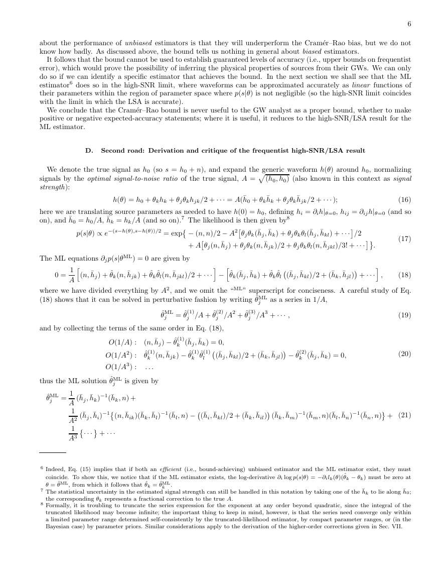
D. Second road: Derivation and critique of the frequentist high-SNR/LSA result
We denote the true signal as h0 (so s = h0 + n), and expand the generic waveform h(θ) around h0, normalizing
(h0, h0) (also known in this context as signal
signals by the optimal signal-to-noise ratio of the true signal, A =
strength):
h(θ) = h0 + θkhk + θjθkhjk/2 + ··· = A(¯h0 + θk¯hk + θjθk¯hjk/2 + ··· );
(16)
here we are translating source parameters as needed to have h(0) = h0, defining hi = ∂ih|θ=0, hij = ∂ij h|θ=0 (and so
on), and ¯h0 = h0/A, ¯hk = hk/A (and so on).7 The likelihood is then given by8
The ML equations ∂jp(s|θML) = 0 are given by
−(s−h(θ),s−h(θ))/2 = exp
p(s|θ) ∝ e
(n, ¯hj) + ˆθk(n, ¯hjk) + ˆθk ˆθl(n, ¯hjkl)/2 + ···
0 =
1
A
− (n, n)/2 − A2
θjθk(¯hj, ¯hk) + θjθkθl(¯hj, ¯hkl) + ···
θj(n, ¯hj) + θjθk(n, ¯hjk)/2 + θjθkθl(n, ¯hjkl)/3! + ···
+ A
/2
.
ˆθk(¯hj , ¯hk) + ˆθk ˆθl
(¯hj, ¯hkl)/2 + (¯hk, ¯hjl)
−
(17)
(18)
,
+ ···
where we have divided everything by A2, and we omit the “ML” superscript for conciseness. A careful study of Eq.
(18) shows that it can be solved in perturbative fashion by writing ˆθML
as a series in 1/A,
j
j /A + ˆθ
and by collecting the terms of the same order in Eq. (18),
k (¯hj, ¯hk) = 0,
j = ˆθ
ˆθML
(2)
(1)
O(1/A) :
O(1/A2) :
O(1/A3) :
(1)
(n, ¯hj) − ˆθ
k (n, ¯hjk) − ˆθ
ˆθ
. . .
(1)
j /A2 + ˆθ
(3)
j /A3 + ··· ,
− ˆθ
(1)
k
ˆθ
(1)
l
(¯hj, ¯hkl)/2 + (¯hk, ¯hjl)
(2)
k (¯hj, ¯hk) = 0,
thus the ML solution ˆθML
j
is given by
−1(¯hl, n) −
(n, ¯hik)(¯hk, ¯hl)
(¯hi, ¯hkl)/2 + (¯hk, ¯hil)
(¯hk, ¯hm)
−1(¯hm, n)(¯hl, ¯hn)
(19)
(20)
+
(21)
−1(¯hn, n)
ˆθML
j =
1
−1(¯hk, n) +
(¯hj, ¯hk)
A
1
−1
···
A2 (¯hj , ¯hi)
+ ···
1
A3
6 Indeed, Eq. (15) implies that if both an efficient (i.e., bound-achieving) unbiased estimator and the ML estimator exist, they must
coincide. To show this, we notice that if the ML estimator exists, the log-derivative ∂i log p(s|θ) = −∂ilk(θ)(ˆθk − θk) must be zero at
θ = ˆθML, from which it follows that ˆθk = ˆθML
k .
7 The statistical uncertainty in the estimated signal strength can still be handled in this notation by taking one of the ¯hk to lie along ¯h0;
the corresponding θk represents a fractional correction to the true A.
8 Formally, it is troubling to truncate the series expression for the exponent at any order beyond quadratic, since the integral of the
truncated likelihood may become infinite; the important thing to keep in mind, however, is that the series need converge only within
a limited parameter range determined self-consistently by the truncated-likelihood estimator, by compact parameter ranges, or (in the
Bayesian case) by parameter priors. Similar considerations apply to the derivation of the higher-order corrections given in Sec. VII.
�
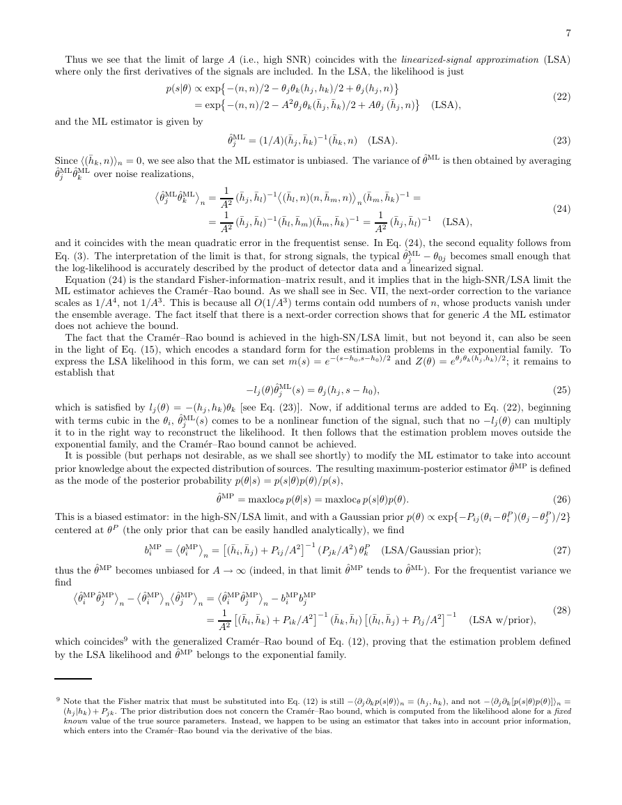
Thus we see that the limit of large A (i.e., high SNR) coincides with the linearized-signal approximation (LSA)
where only the first derivatives of the signals are included. In the LSA, the likelihood is just
−(n, n)/2 − θjθk(hj , hk)/2 + θj(hj, n)
−(n, n)/2 − A2θjθk(¯hj, ¯hk)/2 + Aθj (¯hj, n)
p(s|θ) ∝ exp
= exp
(LSA),
(22)
7
and the ML estimator is given by
(23)
Since (¯hk, n)n = 0, we see also that the ML estimator is unbiased. The variance of ˆθML is then obtained by averaging
ˆθML
over noise realizations,
(LSA).
ˆθML
j = (1/A)(¯hj , ¯hk)
ˆθML
j
k
−1(¯hk, n)
ˆθML
j
ˆθML
k
n =
=
1
−1
A2 (¯hj, ¯hl)
1
A2 (¯hj, ¯hl)
(¯hl, n)(n, ¯hm, n)
−1(¯hl, ¯hm)(¯hm, ¯hk)
n(¯hm, ¯hk)
−1 =
−1 =
1
−1
A2 (¯hj , ¯hl)
(LSA),
(24)
and it coincides with the mean quadratic error in the frequentist sense. In Eq. (24), the second equality follows from
j − θ0j becomes small enough that
Eq. (3). The interpretation of the limit is that, for strong signals, the typical ˆθML
the log-likelihood is accurately described by the product of detector data and a linearized signal.
Equation (24) is the standard Fisher-information–matrix result, and it implies that in the high-SNR/LSA limit the
ML estimator achieves the Cram´er–Rao bound. As we shall see in Sec. VII, the next-order correction to the variance
scales as 1/A4, not 1/A3. This is because all O(1/A3) terms contain odd numbers of n, whose products vanish under
the ensemble average. The fact itself that there is a next-order correction shows that for generic A the ML estimator
does not achieve the bound.
The fact that the Cram´er–Rao bound is achieved in the high-SN/LSA limit, but not beyond it, can also be seen
in the light of Eq. (15), which encodes a standard form for the estimation problems in the exponential family. To
−(s−h0,s−h0)/2 and Z(θ) = eθjθk(hj ,hk)/2; it remains to
express the LSA likelihood in this form, we can set m(s) = e
establish that
−lj(θ)ˆθML
(s) = θj(hj, s − h0),
j
(25)
which is satisfied by lj(θ) = −(hj, hk)θk [see Eq. (23)]. Now, if additional terms are added to Eq. (22), beginning
(s) comes to be a nonlinear function of the signal, such that no −lj(θ) can multiply
with terms cubic in the θi, ˆθML
it to in the right way to reconstruct the likelihood. It then follows that the estimation problem moves outside the
exponential family, and the Cram´er–Rao bound cannot be achieved.
It is possible (but perhaps not desirable, as we shall see shortly) to modify the ML estimator to take into account
prior knowledge about the expected distribution of sources. The resulting maximum-posterior estimator ˆθMP is defined
as the mode of the posterior probability p(θ|s) = p(s|θ)p(θ)/p(s),
j
This is a biased estimator: in the high-SN/LSA limit, and with a Gaussian prior p(θ) ∝ exp{−Pij(θi−θP
centered at θP (the only prior that can be easily handled analytically), we find
ˆθMP = maxlocθ p(θ|s) = maxlocθ p(s|θ)p(θ).
−1 (Pjk/A2) θP
(¯hi, ¯hj) + Pij /A2
bMP
i =
θMP
i
(27)
thus the ˆθMP becomes unbiased for A → ∞ (indeed, in that limit ˆθMP tends to ˆθML). For the frequentist variance we
find
(LSA/Gaussian prior);
n =
k
i )(θj −θP
(26)
j )/2}
−
ˆθMP
i
ˆθMP
j
n
ˆθMP
i
n
ˆθMP
j
n =
ˆθMP
i
1
A2
=
j
− bMP
ˆθMP
bMP
j
(¯hi, ¯hk) + Pik/A2
−1 (¯hk, ¯hl)
n
i
−1
(¯hl, ¯hj) + Plj /A2
(LSA w/prior),
(28)
which coincides9 with the generalized Cram´er–Rao bound of Eq. (12), proving that the estimation problem defined
by the LSA likelihood and ˆθMP belongs to the exponential family.
9 Note that the Fisher matrix that must be substituted into Eq. (12) is still −∂j ∂kp(s|θ)n = (hj, hk), and not −∂j ∂k[p(s|θ)p(θ)]n =
(hj|hk) + Pjk. The prior distribution does not concern the Cram´er–Rao bound, which is computed from the likelihood alone for a fixed
known value of the true source parameters. Instead, we happen to be using an estimator that takes into in account prior information,
which enters into the Cram´er–Rao bound via the derivative of the bias.
�
The reason why ˆθMP is not too useful to characterize future parameter-estimation performance is that we expect a
reasonable measure of error to converge to the effective width of the prior in the limit of vanishing signal strength.
Instead, in the absence of any information from the experiment, ˆθMP becomes stuck at the mode of the prior, and its
variance [in Eq. (28)] tends to zero. This behavior occurs for any nonuniform prior.10
8
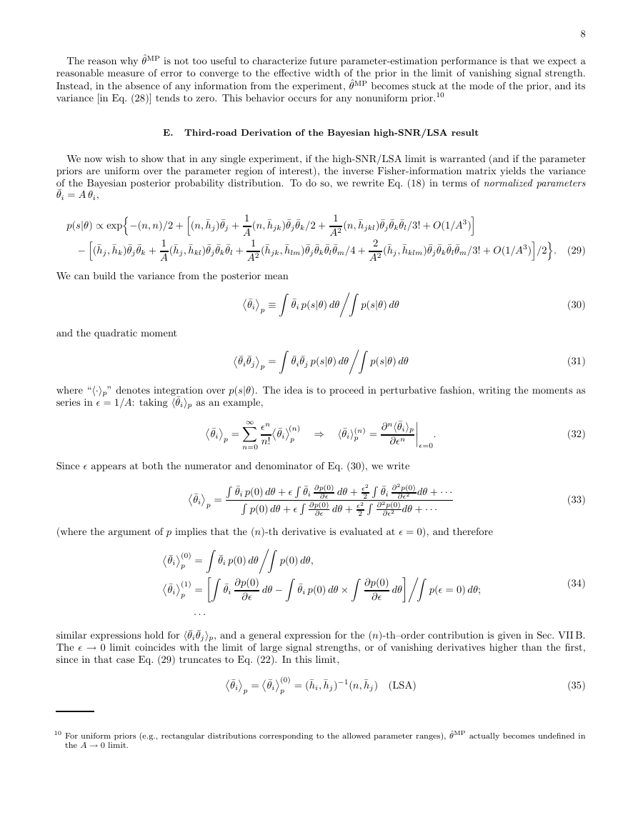
E. Third-road Derivation of the Bayesian high-SNR/LSA result
We now wish to show that in any single experiment, if the high-SNR/LSA limit is warranted (and if the parameter
priors are uniform over the parameter region of interest), the inverse Fisher-information matrix yields the variance
of the Bayesian posterior probability distribution. To do so, we rewrite Eq. (18) in terms of normalized parameters
¯θi = A θi,
p(s|θ) ∝ exp
−
(¯hj , ¯hk)¯θj ¯θk +
−(n, n)/2 +
We can build the variance from the posterior mean
1
A
(n, ¯hj)¯θj +
1
(n, ¯hjk)¯θj ¯θk/2 +
A
1
(¯hj, ¯hkl)¯θj ¯θk ¯θl +
A2 (¯hjk, ¯hlm)¯θj ¯θk ¯θl ¯θm/4 +
≡
¯θi
p
¯θi p(s|θ) dθ
1
A2 (n, ¯hjkl)¯θj ¯θk ¯θl/3! + O(1/A3)
2
A2 (¯hj, ¯hklm)¯θj ¯θk ¯θl ¯θm/3! + O(1/A3)
/2
.
(29)
(30)
and the quadratic moment
¯θi ¯θj
(31)
where “·p” denotes integration over p(s|θ). The idea is to proceed in perturbative fashion, writing the moments as
series in � = 1/A: taking ¯θip as an example,
∞
p =
¯θi ¯θj p(s|θ) dθ
p(s|θ) dθ
⇒ ¯θi(n)
p = ∂n¯θip
∂�n
.
�=0
Since � appears at both the numerator and denominator of Eq. (30), we write
¯θi
p =
n=0
¯θi
p =
¯θi p(0) dθ + �
p(0) dθ + �
∂p(0)
¯θi
∂p(0)
∂� dθ + �2
∂� dθ + �2
2
2
∂2p(0)
¯θi
∂�2 dθ + ···
∂�2 dθ + ···
∂2p(0)
(where the argument of p implies that the (n)-th derivative is evaluated at � = 0), and therefore
p(s|θ) dθ
(n)
p
¯θi
�n
n!
(32)
(33)
(34)
(0)
(1)
¯θi
¯θi
p =
p =
. . .
¯θi p(0) dθ
p(0) dθ,
¯θi
∂p(0)
∂�
dθ −
¯θi p(0) dθ ×
∂p(0)
∂�
dθ
p(� = 0) dθ;
similar expressions hold for ¯θi ¯θjp, and a general expression for the (n)-th–order contribution is given in Sec. VII B.
The � → 0 limit coincides with the limit of large signal strengths, or of vanishing derivatives higher than the first,
since in that case Eq. (29) truncates to Eq. (22). In this limit,
(0)
p = (¯hi, ¯hj)
¯θi
p =
¯θi
−1(n, ¯hj)
(LSA)
(35)
10 For uniform priors (e.g., rectangular distributions corresponding to the allowed parameter ranges), ˆθMP actually becomes undefined in
the A → 0 limit.
�



 2023年江西萍乡中考道德与法治真题及答案.doc
 2012年重庆南川中考生物真题及答案.doc
 2013年江西师范大学地理学综合及文艺理论基础考研真题.doc
 2020年四川甘孜小升初语文真题及答案I卷.doc
 2020年注册岩土工程师专业基础考试真题及答案.doc
 2023-2024学年福建省厦门市九年级上学期数学月考试题及答案.doc
 2021-2022学年辽宁省沈阳市大东区九年级上学期语文期末试题及答案.doc
 2022-2023学年北京东城区初三第一学期物理期末试卷及答案.doc
 2018上半年江西教师资格初中地理学科知识与教学能力真题及答案.doc
 2012年河北国家公务员申论考试真题及答案-省级.doc
 2020-2021学年江苏省扬州市江都区邵樊片九年级上学期数学第一次质量检测试题及答案.doc
 2022下半年黑龙江教师资格证中学综合素质真题及答案.doc