Generalized-ICP
Aleksandr V. Segal
Stanford University
Dirk Haehnel
Stanford University
Sebastian Thrun
Stanford University
Email: avsegal@cs.stanford.edu
Email: haehnel@stanford.edu
Email: thrun@stanford.edu
Abstract— In this paper we combine the Iterative Closest
Point (’ICP’) and ‘point-to-plane ICP‘ algorithms into a single
probabilistic framework. We then use this framework to model
locally planar surface structure from both scans instead of just
the ”model” scan as is typically done with the point-to-plane
method. This can be thought of as ‘plane-to-plane’. The new
approach is tested with both simulated and real-world data and
is shown to outperform both standard ICP and point-to-plane.
Furthermore, the new approach is shown to be more robust to
incorrect correspondences, and thus makes it easier to tune the
maximum match distance parameter present in most variants of
ICP. In addition to the demonstrated performance improvement,
the proposed model allows for more expressive probabilistic
models to be incorporated into the ICP framework. While
maintaining the speed and simplicity of ICP, the Generalized-ICP
could also allow for the addition of outlier terms, measurement
noise, and other probabilistic techniques to increase robustness.
I. INTRODUCTION
Over the last decade, range images have grown in popularity
and found increasing applications in fields including medical
imaging, object modeling, and robotics. Because of occlusion
and limited sensor range, most of these applications require
accurate methods of combining multiple range images into a
single model. Particularly in mobile robotics, the availability
of range sensors capable of quickly capturing an entire 3D
scene has drastically improved the state of the art. A striking
illustration of this is the fact that virtually all competitors in the
DARPA Grand Challenge relied on fast-scanning laser range
finders as the primary input method for obstacle avoidance,
motion planning, and mapping. Although GPS and IMUs are
often used to calculate approximate displacements, they are not
accurate enough to reliably produce precise positioning. In ad-
dition, there are many situation (tunnels, parking garages, tall
buildings) which obstruct GPS reception and further decrease
accuracy. To deal with this shortcoming, most applications
rely on scan-matching of range data to refine the localization.
Despite such wide usage, the typical approach to solving the
scan-matching problem has remained largely unchanged since
its introduction.
II. SCANMATCHING
Originally applied to scan-matching in the early 90s, the
ICP technique has had many variations proposed over the
past decade and a half. Three papers published around the
same time period outline what is still considered the state
of the art solution for scan-matching. The most often cited
analysis of the algorithm comes from Besl and McKay[1]. [1]
directly addresses registration of 3D shapes described either
geometrically or with point clouds. Chen and Medioni[7]
considered the more specific problem of aligning range data
for object modeling. Their approach takes advantage of the
tendency of most range data to be locally planar and intro-
duces the ”point-to-plane” variant of ICP. Zhang[5] almost
simultaneously describes ICP, but adds a robust method of
outlier rejection in the correspondence selection phase of the
algorithm.
Two more modern alternatives are Iterative Dual Correspon-
dence [15] and Metric-Based ICP [16]. IDC improves the
point-matching process by maintaining two sets of correspon-
dences. MbICP is designed to improve convergence with large
initial orientation errors by explicitly putting a measure of
rotational error as part of the distance metric to be minimized.
The primary advantages of most ICP based methods are
simplicity and relatively quick performance when imple-
mented with kd-trees for closest-point look up. The draw-
backs include the implicit assumption of full overlap of the
shapes being matched and the theoretical requirement that the
points are taken from a known geometric surface rather than
measured [1]. The first assumption is violated by partially
overlapped scans (taken from different locations). The sec-
ond causes problems because different discretizations of the
physical surface make it impossible to get exact overlap of
the individual points even after convergence. Point-to-plane,
as suggested in [7], solves the discretization problem by not
penalizing offsets along a surface. The full overlap assumption
is usually handled by setting a maximum distance threshold
in the correspondence.
Aside from point-to-plane, most ICP variations use a closed
form solution to iteratively compute the alignment from the
correspondences. This is typically done with [10] or similar
techniques based on cross-correlation of the two data sets. Re-
cently, there has been interest in the use of generic non-linear
optimization techniques instead of the more specific closed
form approaches [9]. These techniques are advantageous in
that they allow for more generic minimization functions rather
then just the sum of euclidean distances. [9] uses non-linear
optimization with robust statistics to show a wider basin of
convergence.
We argue that among these, the probabilistic techniques
are some of the best motivated due to the large amount of
theoretical work already in place to support them. [2] applies
a probabilistic model by assuming the second scan is generated
from the first
through a random process. [4] Applies ray
tracing techniques to maximize the probability of alignment.
�
[8] builds a set of compatible correspondences, and then
maximizes probability of alignment over this distribution. [17]
introduces a fully probabilistic framework which takes into
account a motion model and allows estimates of registration
uncertainty. An interesting aspect of the approach is that a
sampled analog of the Generalized Hough Transform is used
to compute alignment without explicit correspondences, taking
both surface normals into account for 2D data sets.
There is also a large amount of literature devoted to solving
the global alignment problem with multiple scans ([18] and
many others). Many approaches to this ([18] in particular) use
a pair-wise matching algorithm as a basic component. This
makes improvements in pairwise matching applicable to the
global alignment problem as well.
Our approach falls somewhere between standard IPC and
the fully probabilistic models. It
is based on using MLE
as the non-linear optimization step, and computing discrete
correspondences using kd-trees. It is unique in that it provides
symmetry and incorporates the structural assumptions of [7].
Because closest point look up is done with euclidean distance,
however, kd-trees can be used to achieve fast performance
on large pointclouds. This is typically not possible with fully
probabilistic methods as these require computing a MAP
estimate over assignments. In contrast to [8], we argue that
the data should be assumed to be locally planar since most
environments sampled for range data are piecewise smooth
surfaces. By giving the minimization processes a probabilistic
interpretation, we show that is easy to extend the technique to
include structural information from both scans, rather then just
one as is typically done in ”point-to-plane” ICP. We show that
introducing this symmetry improves accuracy and decreases
dependence on parameters.
Unlike the IDC [15] and MbICP [16] algorithms, our
approach is designed to deal with large 3D pointclouds. Even
more fundamentally both of these approaches are somewhat
orthogonal to our technique. Although MbICP suggests an
alternative distance metric (as do we), our metric aims to
take into account structure rather then orientation. Since our
technique does not rely on any particular type (or number) of
correspondences, it would likely be improved by incorporating
a secondary set of correspondences as in IDC.
A key difference between our approach and [17] is the
computational complexity involved. [17] is designed to deal
with planar scan data – the Generalized Hough Transform sug-
gested requires comparing every point in one scan with every
point in the other (or a proportional number of comparisons
in the case of sampling). Our approach works with kd-trees
for closest point look up and thus requires O(n log(n) explicit
point comparisons. It is not clear how to efficiently generalize
the approach in [17] to the datasets considered in this paper.
Furthermore, there are philosophical differences in the models.
This paper proceeds by summarizing the ICP and point-
to-plane algorithms, and then introducing Generalized-ICP
as a natural extension of these two standard approaches.
Experimental results are then presented which highlight the
advantages of Generalized-ICP.
A. ICP
The key concept of the standard ICP algorithm can be
summarized in two steps:
1) compute correspondences between the two scans.
2) compute a transformation which minimizes distance
between corresponding points.
Iteratively repeating these two steps typically results in conver-
gence to the desired transformation. Because we are violating
the assumption of full overlap, we are forced to add a max-
imum matching threshold dmax. This threshold accounts for
the fact that some points will not have any correspondence in
the second scan (e.g. points which are outside the boundary of
scan A). In most implementations of ICP, the choice of dmax
represents a trade off between convergence and accuracy. A
low value results in bad convergence (the algorithm becomes
“short sighted”); a large value causes incorrect correspon-
dences to pull the final alignment away from the correct value.
Standard ICP is listed as Alg. 1.
input : Two pointclouds: A = {ai}, B = {bi}
An initial transformation: T0
and B
output: The correct transformation, T , which aligns A
T ← T0;
while not converged do
for i ← 1 to N do
mi ← FindClosestPointInA(T · bi);
if
||mi − T · bi|| ≤ dmax then
wi ← 1;
wi ← 0;
else
end
{
end
T ← argmin
T
i
end
wi||T · bi − mi||2};
Algorithm 1: Standard ICP
1
2
3
4
5
6
7
8
9
10
11
12
B. Point-to-plane
The point-to-plane variant of ICP improves performance by
taking advantage of surface normal information. Originally
introduced by Chen and Medioni[7], the technique has come
into widespread use as a more robust and accurate variant of
standard ICP when presented with 2.5D range data. Instead
of minimizing Σ||T · bi − mi||2, the point-to-plane algorithm
minimizes error along the surface normal (i.e. the projection
of (T · bi − mi) onto the sub-space spanned by the surface
normal). This improvement is implemented by changing line
11 of Alg. 1 as follows:
T ← argmin
wi||ηi · (T · bi − mi)||2}
{
T
i
where ηi is the surface normal at mi.
�
III. GENERALIZED-ICP
In this case, (2) becomes
i
i
T
d(T)
i
d(T)
i
||d(T)
i
||2
(3)
T = argmin
T
= argmin
T
which is exactly the standard ICP update formula.
With the Generalized-IPC framework in place, however, we
have more freedom in modeling the situation; we are free
i }. As a
to pick any set of covariances for {C A
motivating example, we note that the point-to-plane algorithm
can also be thought of probabilistically.
i } and {C B
The update step in point-to-plane ICP is performed as:
||Pi · di||2}
(4)
{
T = argmin
T
i
where Pi is the projection onto the span of the surface normal
at bi. This minimizes the distance of T · ai from the plane
defined by bi and its surface normal. Since Pi is an orthogonal
T . This means ||Pi · di||2
projection matrix, Pi = Pi
can be reformulated as a quadratic form:
2 = Pi
||Pi · di||2 = (Pi · di)T · (Pi · di)
· Pi · di
Looking at (4) in this format, we get:
= dT
i
{
T = argmin
T
i
· Pi · di}
dT
i
(5)
Observing the similarity between the above and (2), it can
be shown that point-to-plane ICP is a limiting case of
Generalized-ICP. In this case
−1
C B
C A
i = Pi
i = 0
(6)
(7)
Strictly speaking Pi is non-invertible since it is rank defi-
cient. However, if we approximate Pi with an invertible Qi,
Generalized-ICP approaches point-to-plane as Qi → Pi. We
can intuitively interpret this limiting behavior as bi being
constrained along the plane normal vector with nothing known
about its location inside the plane itself.
B. Application: plane-to-plane
In order to improve performance relative to point-to-plane
and increase the symmetry of the model, Generalized-ICP can
be used to take into account surface information from both
scans. The most natural way to incorporate this additional
structure is to include information about the local surface of
the second scan into (7). This captures the intuitive nature
of the situation, but is not mathematically feasible since the
matrices involved are singular. Instead, we use the intuition of
point-to-plane to motivate a probabilistic model.
The insight of the point-to-plane algorithm is that our point
cloud has more structure then an arbitrary set of points in
3-space; it is actually a collection of surfaces sampled by
a range-measuring sensor. This means we are dealing with
A. Derivation
Generalized-ICP is based on attaching a probabilistic model
to the minimization step on line 11 of Alg. 1. The technique
keeps the rest of the algorithm unchanged so as to reduce
complexity and maintain speed. Notably, correspondences are
still computed with the standard Euclidean distance rather then
a probabilistic measure. This is done to allow for the use of
kd-trees in the look up of closest points and hence maintain
the principle advantages of ICP over other fully probabilistic
techniques – speed and simplicity.
Since only line 11 is relevant, we limit the scope of the
derivation to this context. To simplify notation, we assume
that the closest point look up has already been performed
and that the two point clouds, A = {ai}i=1,...,N and B =
{bi}i=1,...,N , are indexed according to their correspondences
(i.e. ai corresponds with bi). For the purpose of this section,
we also assume all correspondences with ||mi−T ·bi|| > dmax
have been removed from the data.
In the probabilistic model we assume the existence of
an underlying set of points, ˆA = { ˆai} and ˆB = { ˆbi},
which generate A and B according to ai ∼ N ( ˆai, C A
i )
i } are
and bi ∼ N ( ˆbi, C B
covariance matrices associated with the measured points. If
we assume perfect correspondences (geometrically consistent
with no errors due to occlusion or sampling), and the correct
transformation, T∗, we know that
ˆbi = T∗ ˆai
i ). In this case, {C A
i } and {C B
(1)
For an arbitrary rigid transformation, T, we define d(T)
i =
bi − Tai, and consider the distribution from which d(T∗)
is drawn. Since ai and bi are assumed to be drawn from
independent Gaussians,
i
d(T∗)
i
∼ N ( ˆbi − (T∗) ˆai, C B
= N (0, C B
i + (T∗)C A
i (T∗)T )
by applying Eq. (1).
Now we use MLE to iteratively compute T by setting
T = argmax
T
p(d(T)
) = argmax
i
log(p(d(T)
i
i + (T∗)C A
i (T∗)T )
T
i
The above can be simplified to
T = argmin
T
i
d(T)
i
T (C B
i + TC A
i TT )−1d(T)
i
This defines the key step of the Generalized-ICP algorithm.
The standard ICP algorithm can be seen as a special case
by setting
C B
C A
i = I
i = 0
i
))
(2)
�
free to move along the y-axis. The incorrect correspondences
thus form very weak and uninformative constraints for the
overall alignment.
Computing the surface covariance matrices requires a sur-
face normal associated with every point in both scans. There
are many techniques for recovering surface normals from point
clouds, and the accuracy of the normals naturally plays an
important role in the performance of the algorithm. In our
implementation, we used PCA on the covariance matrix of the
20 closest points to each scan point. In this case the eigen-
vector associated with the smallest eigenvalue corresponds
with the surface normal. This method is used to compute
the normals for both point-to-plane and Generalized-ICP. For
Generalized-ICP, the rotation matrices are constructed so that
the � component of the variance lines up with the surface
normal.1
IV. RESULTS
We compare all three algorithms to test performance of the
proposed technique. Although efficient closed form solutions
exist for T in standard ICP, we implemented the minimization
with conjugate gradients to simplify comparison. Performance
is analyzed in terms of convergence to the correct solution after
a known offset is introduced between the two scans. We limit
our tests to a maximum of 250 iterations for standard ICP, and
50 iterations for the other two algorithms since convergence
was typically achieved before this point (if at all).
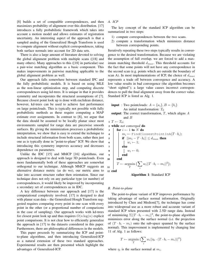
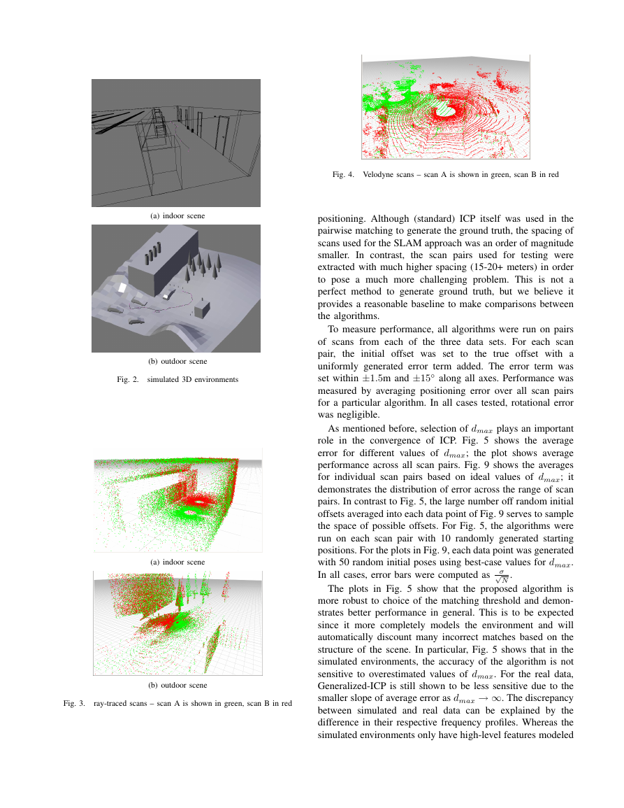
Both simulated (Fig. 3) and real (Fig. 4) data was used in or-
der to demonstrate both theoretical and practical performance.
The simulated data set also allowed tests to be performed on
a wider range of environments with absolutely known ground
truth. The outdoor simulated environment differs from the
collected data primarily in the amount of occlusion presented,
and in the more hilly features of the ground plane. The real-
world outdoor tests also demonstrate performance with more
detailed features and more representative measurement noise.
Simulated data was generated by ray-tracing a SICK scanner
mounted on a rotating joint. Two 3D environments were
created to test performance against absolute ground truth both
in the indoor (Fig. 2(a)) and an outdoor (Fig. 2(b)) scenario.
The indoor environment was based on an office hallway,
while the outdoor setting reflects a typical landscape around a
building. In both cases, we simulated a laser-scanner equipped
robot traveling along a trajectory and taking measurements at
fixed points along the path. Gaussian noise was added to make
the tests more realistic.
Tests were also performed on real data from the logs of
an instrumented car. The logs included data recorded by a
roof-mounted Velodyne range finder as the car made a loop
through a suburban environment and were annotated with GPS
and IMU data. This made it possible to apply a pairwise
constraint-based SLAM technique to generate ground truth
1In our implementation we compute these transformations by considering
the eigen decomposition of the empirical covariance of the 20 closest points,
ˆΣ = UDUT . We then use U in place of the rotation matrix (in effect
replacing D with diag(�, 1, 1) to get the final surface-aligned matrix).
Fig. 1.
illustration of plane-to-plane
a sampled 2-manifold in 3-space. Since real-world surfaces
are at least piece-wise differentiable, we can assume that our
dataset is locally planar. Furthermore, since we are sampling
the manifold from two different perspectives, we will not in
general sample the exact same point (i.e. the correspondence
will never be exact). In essence, every measured point only
provides a constraint along its surface normal. To model this
structure, we consider each sampled point to be distributed
with high covariance along its local plane, and very low
covariance in the surface normal direction. In the case of a
point with e1 as its surface normal, the covariance matrix
becomes
�
0
0 1
0 0
0
0
1
where � is a small constant representing covariance along the
normal. This corresponds to knowing the position along the
normal with very high confidence, but being unsure about its
location in the plane. We model both ai and bi as being drawn
from this sort of distribution.
i and C A
Explicitly, given µi and νi – the respective normal vectors at
bi and ai – C B
i are computed by rotating the above
covariance matrix so that the � term represents uncertainty
along the surface normal. Letting Rx denote one of the
rotations which transform the basis vector e1 → x, set
�
�
0
0 1
0 0
0
0 1
0 0
· RT
· RT
νi
µi
0
0
1
0
0
1
i = Rµi ·
C B
i = Rνi ·
C A
The transformation, T, is then computed via (2).
Fig. 1 provides an illustration of the effect of the algorithm
in an extreme situation. In this case all of the points along the
vertical section of the green scan are incorrectly associated
with a single point
in the red scan. Because the surface
orientations are inconsistent, plane-to-plane will automatically
discount these matches: the final summed covariance matrix
of each correspondence will be isotropic and will form a very
small contribution to the objective function relative to the thin
and sharply defined correspondence covariance matrices. An
alternative view of this behavior is as a soft constraint for each
correspondence. The inconsistent matches allow the red scan-
point to move along the x-axis while the green scan-points are
�
(a) indoor scene
(b) outdoor scene
Fig. 2.
simulated 3D environments
(a) indoor scene
(b) outdoor scene
Fig. 3.
ray-traced scans – scan A is shown in green, scan B in red
Fig. 4. Velodyne scans – scan A is shown in green, scan B in red
positioning. Although (standard) ICP itself was used in the
pairwise matching to generate the ground truth, the spacing of
scans used for the SLAM approach was an order of magnitude
smaller. In contrast,
the scan pairs used for testing were
extracted with much higher spacing (15-20+ meters) in order
to pose a much more challenging problem. This is not a
perfect method to generate ground truth, but we believe it
provides a reasonable baseline to make comparisons between
the algorithms.
the initial offset was set
To measure performance, all algorithms were run on pairs
of scans from each of the three data sets. For each scan
pair,
to the true offset with a
uniformly generated error term added. The error term was
set within ±1.5m and ±15◦ along all axes. Performance was
measured by averaging positioning error over all scan pairs
for a particular algorithm. In all cases tested, rotational error
was negligible.
As mentioned before, selection of dmax plays an important
role in the convergence of ICP. Fig. 5 shows the average
error for different values of dmax; the plot shows average
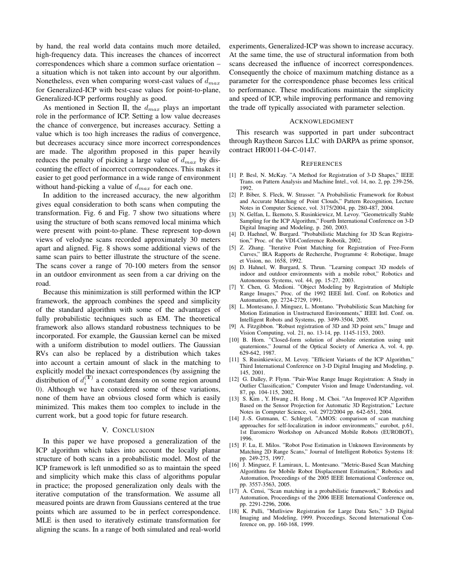
performance across all scan pairs. Fig. 9 shows the averages
for individual scan pairs based on ideal values of dmax; it
demonstrates the distribution of error across the range of scan
pairs. In contrast to Fig. 5, the large number off random initial
offsets averaged into each data point of Fig. 9 serves to sample
the space of possible offsets. For Fig. 5, the algorithms were
run on each scan pair with 10 randomly generated starting
positions. For the plots in Fig. 9, each data point was generated
with 50 random initial poses using best-case values for dmax.
In all cases, error bars were computed as σ√
.
N
The plots in Fig. 5 show that the proposed algorithm is
more robust to choice of the matching threshold and demon-
strates better performance in general. This is to be expected
since it more completely models the environment and will
automatically discount many incorrect matches based on the
structure of the scene. In particular, Fig. 5 shows that in the
simulated environments, the accuracy of the algorithm is not
sensitive to overestimated values of dmax. For the real data,
Generalized-ICP is still shown to be less sensitive due to the
smaller slope of average error as dmax → ∞. The discrepancy
between simulated and real data can be explained by the
difference in their respective frequency profiles. Whereas the
simulated environments only have high-level features modeled
�
(a) simulated indoor
(b) simulated outdoor
(c) Velodyne data
Fig. 5.
average error as a function of dmax
(a) Initial alignment
(b) Point-to-plane
(c) Generalized-ICP
Fig. 6. Example of results for velodyne scan pair #31
(a) Initial alignment
(b) Point-to-plane
(c) Generalized-ICP
Fig. 7. Example of results for velodyne scan pair #45
0 0.2 0.4 0.6 0.8 1 1.2 0 0.5 1 1.5 2 2.5 3 3.5 4 4.5 5average error [m]max. match distance [m]Simulated Hallway with 15,000 points, 1cm noiseGeneralized ICPPoint-to-plane ICPStandard ICP 0 0.2 0.4 0.6 0.8 1 1.2 0 0.5 1 1.5 2 2.5 3 3.5 4 4.5 5average error [m]max. match distance [m]Simulated Outdoor with 15,000 points, 1cm noiseGeneralized ICPPoint-to-plane ICPStandard ICP 0 0.5 1 1.5 2 0 0.5 1 1.5 2 2.5 3 3.5 4 4.5 5average error [m]max. match distance [m]Velodyne Data with 15,000 pointsGeneralized ICPPoint-to-plane ICPStandard ICP�
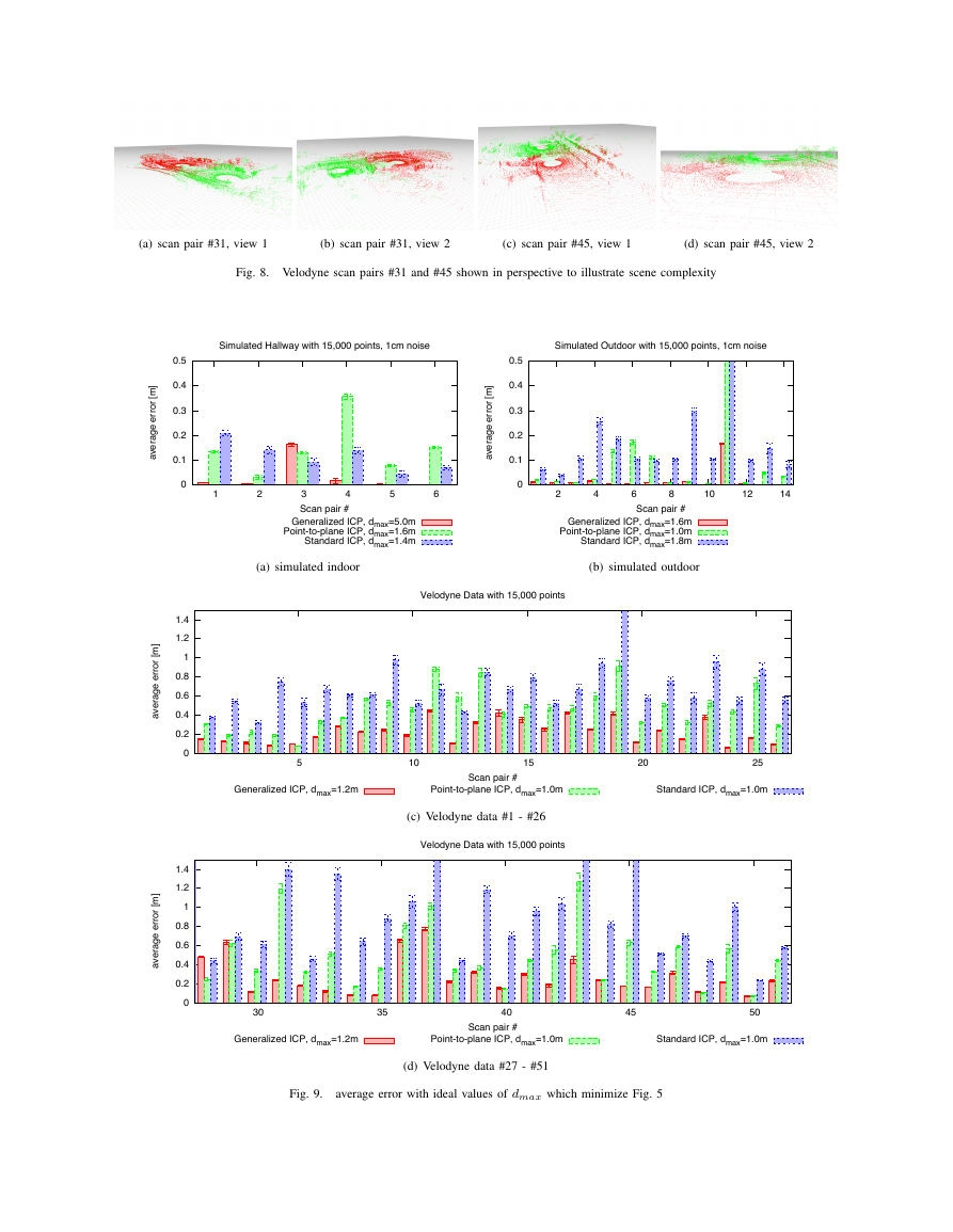
(a) scan pair #31, view 1
(b) scan pair #31, view 2
(c) scan pair #45, view 1
(d) scan pair #45, view 2
Fig. 8. Velodyne scan pairs #31 and #45 shown in perspective to illustrate scene complexity
(a) simulated indoor
(b) simulated outdoor
(c) Velodyne data #1 - #26
(d) Velodyne data #27 - #51
Fig. 9.
average error with ideal values of dmax which minimize Fig. 5
0 0.1 0.2 0.3 0.4 0.5 1 2 3 4 5 6average error [m]Scan pair #Simulated Hallway with 15,000 points, 1cm noiseGeneralized ICP, dmax=5.0mPoint-to-plane ICP, dmax=1.6mStandard ICP, dmax=1.4m 0 0.1 0.2 0.3 0.4 0.5 2 4 6 8 10 12 14average error [m]Scan pair #Simulated Outdoor with 15,000 points, 1cm noiseGeneralized ICP, dmax=1.6mPoint-to-plane ICP, dmax=1.0mStandard ICP, dmax=1.8m 0 0.2 0.4 0.6 0.8 1 1.2 1.4 5 10 15 20 25average error [m]Scan pair #Velodyne Data with 15,000 pointsGeneralized ICP, dmax=1.2mPoint-to-plane ICP, dmax=1.0mStandard ICP, dmax=1.0m 0 0.2 0.4 0.6 0.8 1 1.2 1.4 30 35 40 45 50average error [m]Scan pair #Velodyne Data with 15,000 pointsGeneralized ICP, dmax=1.2mPoint-to-plane ICP, dmax=1.0mStandard ICP, dmax=1.0m�
by hand, the real world data contains much more detailed,
high-frequency data. This increases the chances of incorrect
correspondences which share a common surface orientation –
a situation which is not taken into account by our algorithm.
Nonetheless, even when comparing worst-cast values of dmax
for Generalized-ICP with best-case values for point-to-plane,
Generalized-ICP performs roughly as good.
As mentioned in Section II, the dmax plays an important
role in the performance of ICP. Setting a low value decreases
the chance of convergence, but increases accuracy. Setting a
value which is too high increases the radius of convergence,
but decreases accuracy since more incorrect correspondences
are made. The algorithm proposed in this paper heavily
reduces the penalty of picking a large value of dmax by dis-
counting the effect of incorrect correspondences. This makes it
easier to get good performance in a wide range of environment
without hand-picking a value of dmax for each one.
In addition to the increased accuracy, the new algorithm
gives equal consideration to both scans when computing the
transformation. Fig. 6 and Fig. 7 show two situations where
using the structure of both scans removed local minima which
were present with point-to-plane. These represent top-down
views of velodyne scans recorded approximately 30 meters
apart and aligned. Fig. 8 shows some additional views of the
same scan pairs to better illustrate the structure of the scene.
The scans cover a range of 70-100 meters from the sensor
in an outdoor environment as seen from a car driving on the
road.
Because this minimization is still performed within the ICP
framework, the approach combines the speed and simplicity
of the standard algorithm with some of the advantages of
fully probabilistic techniques such as EM. The theoretical
framework also allows standard robustness techniques to be
incorporated. For example, the Gaussian kernel can be mixed
with a uniform distribution to model outliers. The Gaussian
RVs can also be replaced by a distribution which takes
into account a certain amount of slack in the matching to
explicitly model the inexact correspondences (by assigning the
distribution of d(T)
a constant density on some region around
0). Although we have considered some of these variations,
none of them have an obvious closed form which is easily
minimized. This makes them too complex to include in the
current work, but a good topic for future research.
i
V. CONCLUSION
In this paper we have proposed a generalization of the
ICP algorithm which takes into account the locally planar
structure of both scans in a probabilistic model. Most of the
ICP framework is left unmodified so as to maintain the speed
and simplicity which make this class of algorithms popular
in practice; the proposed generalization only deals with the
iterative computation of the transformation. We assume all
measured points are drawn from Gaussians centered at the true
points which are assumed to be in perfect correspondence.
MLE is then used to iteratively estimate transformation for
aligning the scans. In a range of both simulated and real-world
experiments, Generalized-ICP was shown to increase accuracy.
At the same time, the use of structural information from both
scans decreased the influence of incorrect correspondences.
Consequently the choice of maximum matching distance as a
parameter for the correspondence phase becomes less critical
to performance. These modifications maintain the simplicity
and speed of ICP, while improving performance and removing
the trade off typically associated with parameter selection.
ACKNOWLEDGMENT
This research was supported in part under subcontract
through Raytheon Sarcos LLC with DARPA as prime sponsor,
contract HR0011-04-C-0147.
REFERENCES
[1] P. Besl, N. McKay. ”A Method for Registration of 3-D Shapes,” IEEE
Trans. on Pattern Analysis and Machine Intel., vol. 14, no. 2, pp. 239-256,
1992.
[2] P. Biber, S. Fleck, W. Strasser. ”A Probabilistic Framework for Robust
and Accurate Matching of Point Clouds,” Pattern Recognition, Lecture
Notes in Computer Science, vol. 3175/2004, pp. 280-487, 2004.
[3] N. Gelfan, L. Ikemoto, S. Rusinkiewicz, M. Levoy. ”Geometrically Stable
Sampling for the ICP Algorithm,” Fourth International Conference on 3-D
Digital Imaging and Modeling, p. 260, 2003.
[4] D. Haehnel, W. Burgard. ”Probabilistic Matching for 3D Scan Registra-
tion,” Proc. of the VDI-Conference Robotik, 2002.
[5] Z. Zhang. ”Iterative Point Matching for Registration of Free-Form
Curves,” IRA Rapports de Recherche, Programme 4: Robotique, Image
et Vision, no. 1658, 1992.
[6] D. Hahnel, W. Burgard, S. Thrun. ”Learning compact 3D models of
indoor and outdoor environments with a mobile robot,” Robotics and
Autonomous Systems, vol. 44, pp. 15-27, 2003.
[7] Y. Chen, G. Medioni. ”Object Modeling by Registration of Multiple
Range Images,” Proc. of the 1992 IEEE Intl. Conf. on Robotics and
Automation, pp. 2724-2729, 1991.
[8] L. Montesano, J. Minguez, L. Montano. ”Probabilistic Scan Matching for
Motion Estimation in Unstructured Environments,” IEEE Intl. Conf. on.
Intelligent Robots and Systems, pp. 3499-3504, 2005.
[9] A. Fitzgibbon. ”Robust registration of 3D and 3D point sets,” Image and
Vision Computing, vol. 21, no. 13-14, pp. 1145-1153, 2003.
[10] B. Horn. ”Closed-form solution of absolute orientation using unit
quaternions,” Journal of the Optical Society of America A, vol. 4, pp.
629-642, 1987.
[11] S. Rusinkiewicz, M. Levoy. ”Efficient Variants of the ICP Algorithm,”
Third International Conference on 3-D Digital Imaging and Modeling, p.
145, 2001.
[12] G. Dalley, P. Flynn. ”Pair-Wise Range Image Registration: A Study in
Outlier Classification,” Computer Vision and Image Understanding, vol.
87, pp. 104-115, 2002.
[13] S. Kim , Y. Hwang , H. Hong , M. Choi. ”An Improved ICP Algorithm
Based on the Sensor Projection for Automatic 3D Registration,” Lecture
Notes in Computer Science, vol. 2972/2004 pp. 642-651, 2004.
[14] J.-S. Gutmann, C. Schlegel, ”AMOS: comparison of scan matching
approaches for self-localization in indoor environments,” eurobot, p.61,
1st Euromicro Workshop on Advanced Mobile Robots (EUROBOT),
1996.
[15] F. Lu, E. Milos. ”Robot Pose Estimation in Unknown Environments by
Matching 2D Range Scans,” Journal of Intelligent Robotics Systems 18:
pp. 249-275, 1997.
[16] J. Minguez, F. Lamiraux, L. Montesano. ”Metric-Based Scan Matching
Algorithms for Mobile Robot Displacement Estimation,” Robotics and
Automation, Proceedings of the 2005 IEEE International Conference on,
pp. 3557-3563, 2005.
[17] A. Censi, ”Scan matching in a probabilistic framework,” Robotics and
Automation, Proceedings of the 2006 IEEE International Conference on,
pp. 2291-2296, 2006.
[18] K. Pulli, ”Mutliview Registration for Large Data Sets,” 3-D Digital
Imaging and Modeling, 1999. Proceedings. Second International Con-
ference on, pp. 160-168, 1999.
�






 2023年江西萍乡中考道德与法治真题及答案.doc
 2012年重庆南川中考生物真题及答案.doc
 2013年江西师范大学地理学综合及文艺理论基础考研真题.doc
 2020年四川甘孜小升初语文真题及答案I卷.doc
 2020年注册岩土工程师专业基础考试真题及答案.doc
 2023-2024学年福建省厦门市九年级上学期数学月考试题及答案.doc
 2021-2022学年辽宁省沈阳市大东区九年级上学期语文期末试题及答案.doc
 2022-2023学年北京东城区初三第一学期物理期末试卷及答案.doc
 2018上半年江西教师资格初中地理学科知识与教学能力真题及答案.doc
 2012年河北国家公务员申论考试真题及答案-省级.doc
 2020-2021学年江苏省扬州市江都区邵樊片九年级上学期数学第一次质量检测试题及答案.doc
 2022下半年黑龙江教师资格证中学综合素质真题及答案.doc