ANSYS Fluent Theory Guide
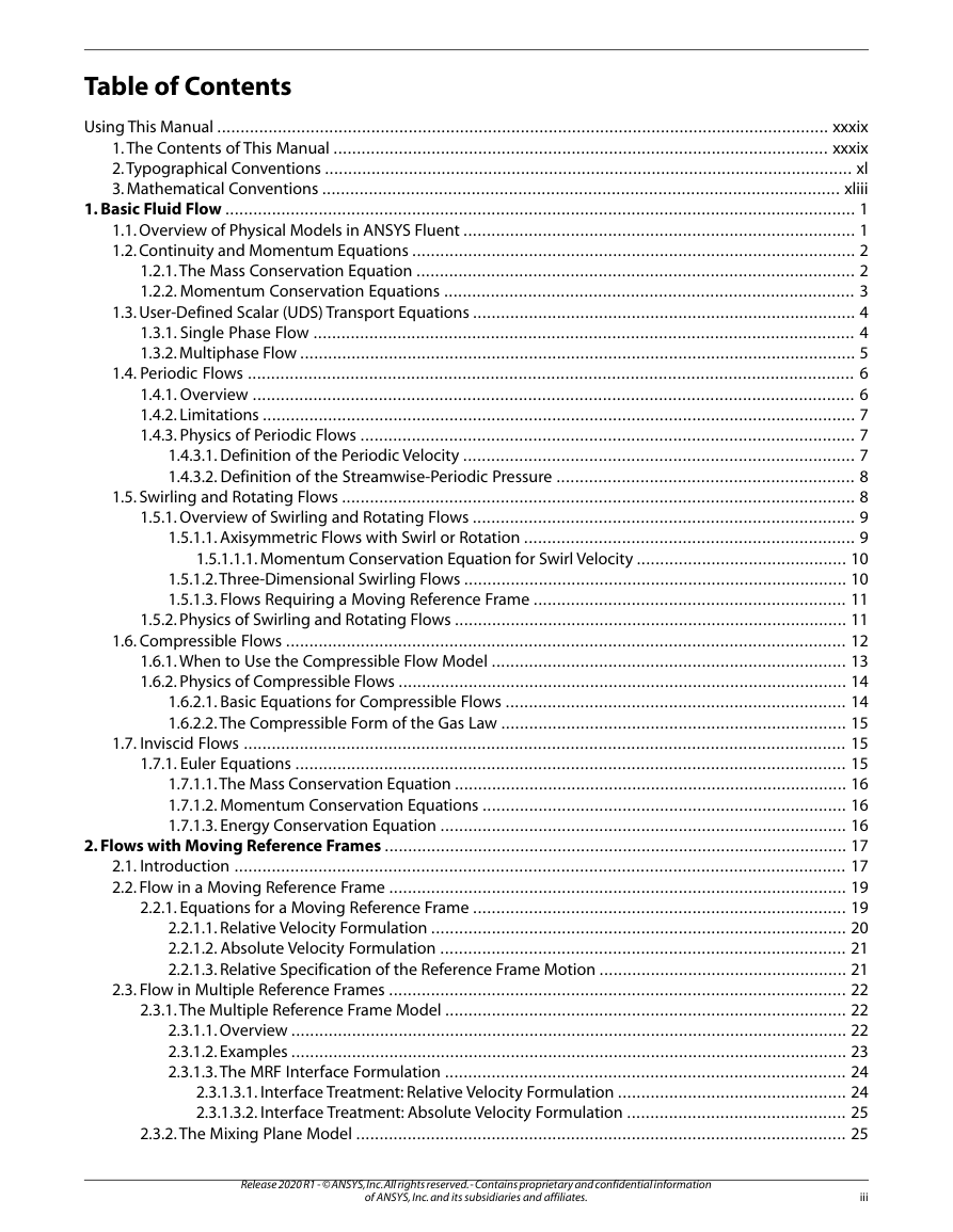
Table of Contents
Using This Manual
1. The Contents of This Manual
2. Typographical Conventions
3. Mathematical Conventions
Chapter 1: Basic Fluid Flow
1.1. Overview of Physical Models in ANSYS Fluent
1.2. Continuity and Momentum Equations
1.2.1. The Mass Conservation Equation
1.2.2. Momentum Conservation Equations
1.3. User-Defined Scalar (UDS) Transport Equations
1.3.1. Single Phase Flow
1.3.2. Multiphase Flow
1.4. Periodic Flows
1.4.1. Overview
1.4.2. Limitations
1.4.3. Physics of Periodic Flows
1.4.3.1. Definition of the Periodic Velocity
1.4.3.2. Definition of the Streamwise-Periodic Pressure
1.5. Swirling and Rotating Flows
1.5.1. Overview of Swirling and Rotating Flows
1.5.1.1. Axisymmetric Flows with Swirl or Rotation
1.5.1.1.1. Momentum Conservation Equation for Swirl Velocity
1.5.1.2. Three-Dimensional Swirling Flows
1.5.1.3. Flows Requiring a Moving Reference Frame
1.5.2. Physics of Swirling and Rotating Flows
1.6. Compressible Flows
1.6.1. When to Use the Compressible Flow Model
1.6.2. Physics of Compressible Flows
1.6.2.1. Basic Equations for Compressible Flows
1.6.2.2. The Compressible Form of the Gas Law
1.7. Inviscid Flows
1.7.1. Euler Equations
1.7.1.1. The Mass Conservation Equation
1.7.1.2. Momentum Conservation Equations
1.7.1.3. Energy Conservation Equation
Chapter 2: Flows with Moving Reference Frames
2.1. Introduction
2.2. Flow in a Moving Reference Frame
2.2.1. Equations for a Moving Reference Frame
2.2.1.1. Relative Velocity Formulation
2.2.1.2. Absolute Velocity Formulation
2.2.1.3. Relative Specification of the Reference Frame Motion
2.3. Flow in Multiple Reference Frames
2.3.1. The Multiple Reference Frame Model
2.3.1.1. Overview
2.3.1.2. Examples
2.3.1.3. The MRF Interface Formulation
2.3.1.3.1. Interface Treatment: Relative Velocity Formulation
2.3.1.3.2. Interface Treatment: Absolute Velocity Formulation
2.3.2. The Mixing Plane Model
2.3.2.1. Overview
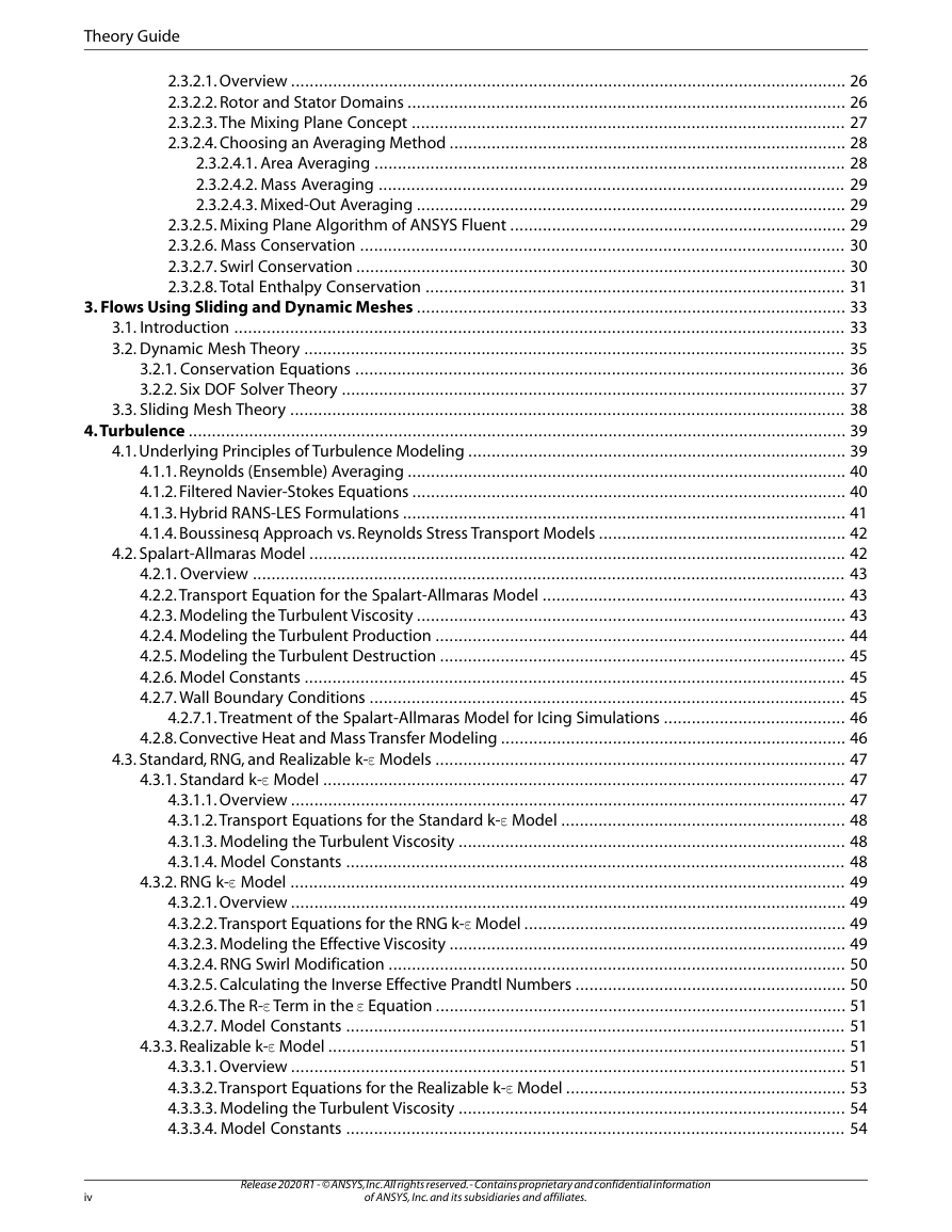
2.3.2.2. Rotor and Stator Domains
2.3.2.3. The Mixing Plane Concept
2.3.2.4. Choosing an Averaging Method
2.3.2.4.1. Area Averaging
2.3.2.4.2. Mass Averaging
2.3.2.4.3. Mixed-Out Averaging
2.3.2.5. Mixing Plane Algorithm of ANSYS Fluent
2.3.2.6. Mass Conservation
2.3.2.7. Swirl Conservation
2.3.2.8. Total Enthalpy Conservation
Chapter 3: Flows Using Sliding and Dynamic Meshes
3.1. Introduction
3.2. Dynamic Mesh Theory
3.2.1. Conservation Equations
3.2.2. Six DOF Solver Theory
3.3. Sliding Mesh Theory
Chapter 4: Turbulence
4.1. Underlying Principles of Turbulence Modeling
4.1.1. Reynolds (Ensemble) Averaging
4.1.2. Filtered Navier-Stokes Equations
4.1.3. Hybrid RANS-LES Formulations
4.1.4. Boussinesq Approach vs. Reynolds Stress Transport Models
4.2. Spalart-Allmaras Model
4.2.1. Overview
4.2.2. Transport Equation for the Spalart-Allmaras Model
4.2.3. Modeling the Turbulent Viscosity
4.2.4. Modeling the Turbulent Production
4.2.5. Modeling the Turbulent Destruction
4.2.6. Model Constants
4.2.7. Wall Boundary Conditions
4.2.7.1. Treatment of the Spalart-Allmaras Model for Icing Simulations
4.2.8. Convective Heat and Mass Transfer Modeling
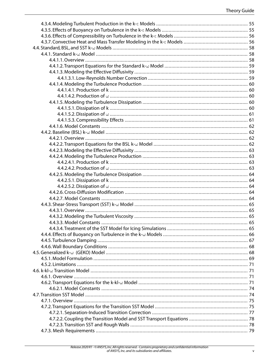
4.3. Standard, RNG, and Realizable k-ε Models
4.3.1. Standard k-ε Model
4.3.1.1. Overview
4.3.1.2. Transport Equations for the Standard k-ε Model
4.3.1.3. Modeling the Turbulent Viscosity
4.3.1.4. Model Constants
4.3.2. RNG k-ε Model
4.3.2.1. Overview
4.3.2.2. Transport Equations for the RNG k-ε Model
4.3.2.3. Modeling the Effective Viscosity
4.3.2.4. RNG Swirl Modification
4.3.2.5. Calculating the Inverse Effective Prandtl Numbers
4.3.2.6. The R-ε Term in the ε Equation
4.3.2.7. Model Constants
4.3.3. Realizable k-ε Model
4.3.3.1. Overview
4.3.3.2. Transport Equations for the Realizable k-ε Model
4.3.3.3. Modeling the Turbulent Viscosity
4.3.3.4. Model Constants
4.3.4. Modeling Turbulent Production in the k-ε Models
4.3.5. Effects of Buoyancy on Turbulence in the k-ε Models
4.3.6. Effects of Compressibility on Turbulence in the k-ε Models
4.3.7. Convective Heat and Mass Transfer Modeling in the k-ε Models
4.4. Standard, BSL, and SST k-ω Models
4.4.1. Standard k-ω Model
4.4.1.1. Overview
4.4.1.2. Transport Equations for the Standard k-ω Model
4.4.1.3. Modeling the Effective Diffusivity
4.4.1.3.1. Low-Reynolds Number Correction
4.4.1.4. Modeling the Turbulence Production
4.4.1.4.1. Production of k
4.4.1.4.2. Production of ω
4.4.1.5. Modeling the Turbulence Dissipation
4.4.1.5.1. Dissipation of k
4.4.1.5.2. Dissipation of ω
4.4.1.5.3. Compressibility Effects
4.4.1.6. Model Constants
4.4.2. Baseline (BSL) k-ω Model
4.4.2.1. Overview
4.4.2.2. Transport Equations for the BSL k-ω Model
4.4.2.3. Modeling the Effective Diffusivity
4.4.2.4. Modeling the Turbulence Production
4.4.2.4.1. Production of k
4.4.2.4.2. Production of ω
4.4.2.5. Modeling the Turbulence Dissipation
4.4.2.5.1. Dissipation of k
4.4.2.5.2. Dissipation of ω
4.4.2.6. Cross-Diffusion Modification
4.4.2.7. Model Constants
4.4.3. Shear-Stress Transport (SST) k-ω Model
4.4.3.1. Overview
4.4.3.2. Modeling the Turbulent Viscosity
4.4.3.3. Model Constants
4.4.3.4. Treatment of the SST Model for Icing Simulations
4.4.4. Effects of Buoyancy on Turbulence in the k-ω Models
4.4.5. Turbulence Damping
4.4.6. Wall Boundary Conditions
4.5. Generalized k-ω (GEKO) Model
4.5.1. Model Formulation
4.5.2. Limitations
4.6. k-kl-ω Transition Model
4.6.1. Overview
4.6.2. Transport Equations for the k-kl-ω Model
4.6.2.1. Model Constants
4.7. Transition SST Model
4.7.1. Overview
4.7.2. Transport Equations for the Transition SST Model
4.7.2.1. Separation-Induced Transition Correction
4.7.2.2. Coupling the Transition Model and SST Transport Equations
4.7.2.3. Transition SST and Rough Walls
4.7.3. Mesh Requirements
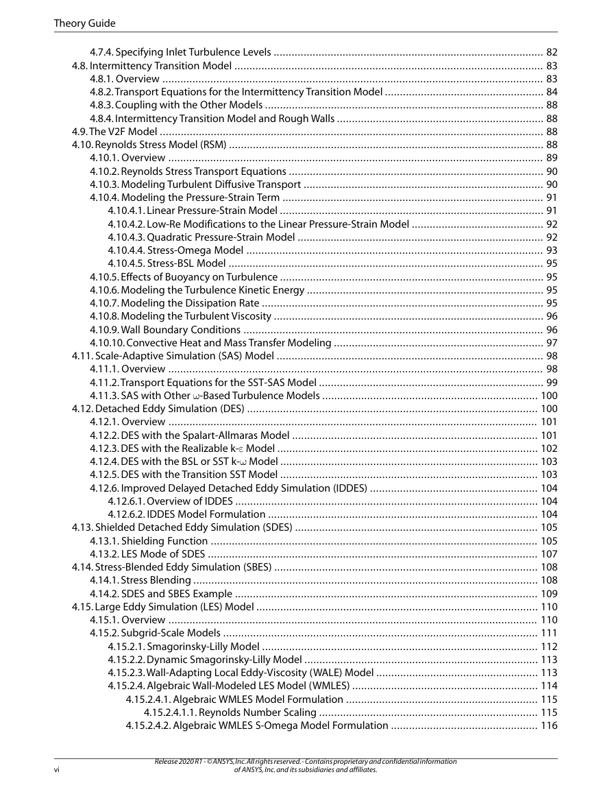
4.7.4. Specifying Inlet Turbulence Levels
4.8. Intermittency Transition Model
4.8.1. Overview
4.8.2. Transport Equations for the Intermittency Transition Model
4.8.3. Coupling with the Other Models
4.8.4. Intermittency Transition Model and Rough Walls
4.9. The V2F Model
4.10. Reynolds Stress Model (RSM)
4.10.1. Overview
4.10.2. Reynolds Stress Transport Equations
4.10.3. Modeling Turbulent Diffusive Transport
4.10.4. Modeling the Pressure-Strain Term
4.10.4.1. Linear Pressure-Strain Model
4.10.4.2. Low-Re Modifications to the Linear Pressure-Strain Model
4.10.4.3. Quadratic Pressure-Strain Model
4.10.4.4. Stress-Omega Model
4.10.4.5. Stress-BSL Model
4.10.5. Effects of Buoyancy on Turbulence
4.10.6. Modeling the Turbulence Kinetic Energy
4.10.7. Modeling the Dissipation Rate
4.10.8. Modeling the Turbulent Viscosity
4.10.9. Wall Boundary Conditions
4.10.10. Convective Heat and Mass Transfer Modeling
4.11. Scale-Adaptive Simulation (SAS) Model
4.11.1. Overview
4.11.2. Transport Equations for the SST-SAS Model
4.11.3. SAS with Other ω-Based Turbulence Models
4.12. Detached Eddy Simulation (DES)
4.12.1. Overview
4.12.2. DES with the Spalart-Allmaras Model
4.12.3. DES with the Realizable k-ε Model
4.12.4. DES with the BSL or SST k-ω Model
4.12.5. DES with the Transition SST Model
4.12.6. Improved Delayed Detached Eddy Simulation (IDDES)
4.12.6.1. Overview of IDDES
4.12.6.2. IDDES Model Formulation
4.13. Shielded Detached Eddy Simulation (SDES)
4.13.1. Shielding Function
4.13.2. LES Mode of SDES
4.14. Stress-Blended Eddy Simulation (SBES)
4.14.1. Stress Blending
4.14.2. SDES and SBES Example
4.15. Large Eddy Simulation (LES) Model
4.15.1. Overview
4.15.2. Subgrid-Scale Models
4.15.2.1. Smagorinsky-Lilly Model
4.15.2.2. Dynamic Smagorinsky-Lilly Model
4.15.2.3. Wall-Adapting Local Eddy-Viscosity (WALE) Model
4.15.2.4. Algebraic Wall-Modeled LES Model (WMLES)
4.15.2.4.1. Algebraic WMLES Model Formulation
4.15.2.4.1.1. Reynolds Number Scaling
4.15.2.4.2. Algebraic WMLES S-Omega Model Formulation
4.15.2.5. Dynamic Kinetic Energy Subgrid-Scale Model
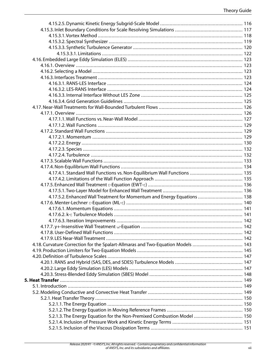
4.15.3. Inlet Boundary Conditions for Scale Resolving Simulations
4.15.3.1. Vortex Method
4.15.3.2. Spectral Synthesizer
4.15.3.3. Synthetic Turbulence Generator
4.15.3.3.1. Limitations
4.16. Embedded Large Eddy Simulation (ELES)
4.16.1. Overview
4.16.2. Selecting a Model
4.16.3. Interfaces Treatment
4.16.3.1. RANS-LES Interface
4.16.3.2. LES-RANS Interface
4.16.3.3. Internal Interface Without LES Zone
4.16.3.4. Grid Generation Guidelines
4.17. Near-Wall Treatments for Wall-Bounded Turbulent Flows
4.17.1. Overview
4.17.1.1. Wall Functions vs. Near-Wall Model
4.17.1.2. Wall Functions
4.17.2. Standard Wall Functions
4.17.2.1. Momentum
4.17.2.2. Energy
4.17.2.3. Species
4.17.2.4. Turbulence
4.17.3. Scalable Wall Functions
4.17.4. Non-Equilibrium Wall Functions
4.17.4.1. Standard Wall Functions vs. Non-Equilibrium Wall Functions
4.17.4.2. Limitations of the Wall Function Approach
4.17.5. Enhanced Wall Treatment ε-Equation (EWT-ε)
4.17.5.1. Two-Layer Model for Enhanced Wall Treatment
4.17.5.2. Enhanced Wall Treatment for Momentum and Energy Equations
4.17.6. Menter-Lechner ε-Equation (ML-ε)
4.17.6.1. Momentum Equations
4.17.6.2. k-ε Turbulence Models
4.17.6.3. Iteration Improvements
4.17.7. y+-Insensitive Wall Treatment ω-Equation
4.17.8. User-Defined Wall Functions
4.17.9. LES Near-Wall Treatment
4.18. Curvature Correction for the Spalart-Allmaras and Two-Equation Models
4.19. Production Limiters for Two-Equation Models
4.20. Definition of Turbulence Scales
4.20.1. RANS and Hybrid (SAS, DES, and SDES) Turbulence Models
4.20.2. Large Eddy Simulation (LES) Models
4.20.3. Stress-Blended Eddy Simulation (SBES) Model
Chapter 5: Heat Transfer
5.1. Introduction
5.2. Modeling Conductive and Convective Heat Transfer
5.2.1. Heat Transfer Theory
5.2.1.1. The Energy Equation
5.2.1.2. The Energy Equation in Moving Reference Frames
5.2.1.3. The Energy Equation for the Non-Premixed Combustion Model
5.2.1.4. Inclusion of Pressure Work and Kinetic Energy Terms
5.2.1.5. Inclusion of the Viscous Dissipation Terms
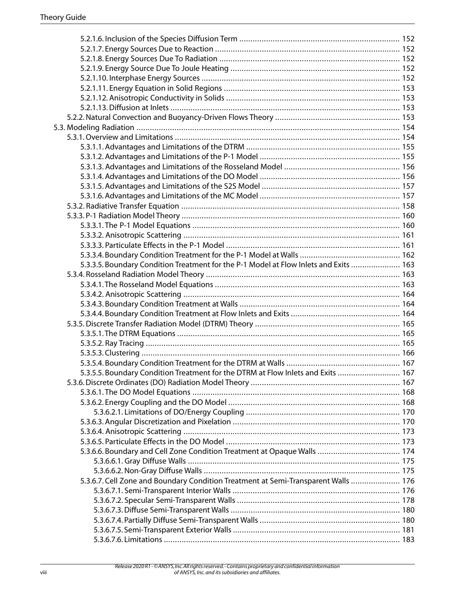
5.2.1.6. Inclusion of the Species Diffusion Term
5.2.1.7. Energy Sources Due to Reaction
5.2.1.8. Energy Sources Due To Radiation
5.2.1.9. Energy Source Due To Joule Heating
5.2.1.10. Interphase Energy Sources
5.2.1.11. Energy Equation in Solid Regions
5.2.1.12. Anisotropic Conductivity in Solids
5.2.1.13. Diffusion at Inlets
5.2.2. Natural Convection and Buoyancy-Driven Flows Theory
5.3. Modeling Radiation
5.3.1. Overview and Limitations
5.3.1.1. Advantages and Limitations of the DTRM
5.3.1.2. Advantages and Limitations of the P-1 Model
5.3.1.3. Advantages and Limitations of the Rosseland Model
5.3.1.4. Advantages and Limitations of the DO Model
5.3.1.5. Advantages and Limitations of the S2S Model
5.3.1.6. Advantages and Limitations of the MC Model
5.3.2. Radiative Transfer Equation
5.3.3. P-1 Radiation Model Theory
5.3.3.1. The P-1 Model Equations
5.3.3.2. Anisotropic Scattering
5.3.3.3. Particulate Effects in the P-1 Model
5.3.3.4. Boundary Condition Treatment for the P-1 Model at Walls
5.3.3.5. Boundary Condition Treatment for the P-1 Model at Flow Inlets and Exits
5.3.4. Rosseland Radiation Model Theory
5.3.4.1. The Rosseland Model Equations
5.3.4.2. Anisotropic Scattering
5.3.4.3. Boundary Condition Treatment at Walls
5.3.4.4. Boundary Condition Treatment at Flow Inlets and Exits
5.3.5. Discrete Transfer Radiation Model (DTRM) Theory
5.3.5.1. The DTRM Equations
5.3.5.2. Ray Tracing
5.3.5.3. Clustering
5.3.5.4. Boundary Condition Treatment for the DTRM at Walls
5.3.5.5. Boundary Condition Treatment for the DTRM at Flow Inlets and Exits
5.3.6. Discrete Ordinates (DO) Radiation Model Theory
5.3.6.1. The DO Model Equations
5.3.6.2. Energy Coupling and the DO Model
5.3.6.2.1. Limitations of DO/Energy Coupling
5.3.6.3. Angular Discretization and Pixelation
5.3.6.4. Anisotropic Scattering
5.3.6.5. Particulate Effects in the DO Model
5.3.6.6. Boundary and Cell Zone Condition Treatment at Opaque Walls
5.3.6.6.1. Gray Diffuse Walls
5.3.6.6.2. Non-Gray Diffuse Walls
5.3.6.7. Cell Zone and Boundary Condition Treatment at Semi-Transparent Walls
5.3.6.7.1. Semi-Transparent Interior Walls
5.3.6.7.2. Specular Semi-Transparent Walls
5.3.6.7.3. Diffuse Semi-Transparent Walls
5.3.6.7.4. Partially Diffuse Semi-Transparent Walls
5.3.6.7.5. Semi-Transparent Exterior Walls
5.3.6.7.6. Limitations
5.3.6.7.7. Solid Semi-Transparent Media
5.3.6.8. Boundary Condition Treatment at Specular Walls and Symmetry Boundaries
5.3.6.9. Boundary Condition Treatment at Periodic Boundaries
5.3.6.10. Boundary Condition Treatment at Flow Inlets and Exits
5.3.7. Surface-to-Surface (S2S) Radiation Model Theory
5.3.7.1. Gray-Diffuse Radiation
5.3.7.2. The S2S Model Equations
5.3.7.3. Clustering
5.3.7.3.1. Clustering and View Factors
5.3.7.3.2. Clustering and Radiosity
5.3.8. Monte Carlo (MC) Radiation Model Theory
5.3.8.1. The MC Model Equations
5.3.8.1.1. Monte Carlo Solution Accuracy
5.3.8.2. Boundary Condition Treatment for the MC Model
5.3.9. Radiation in Combusting Flows
5.3.9.1. The Weighted-Sum-of-Gray-Gases Model
5.3.9.1.1. When the Total (Static) Gas Pressure is Not Equal to 1 atm
5.3.9.2. The Effect of Soot on the Absorption Coefficient
5.3.9.3. The Effect of Particles on the Absorption Coefficient
5.3.10. Choosing a Radiation Model
5.3.10.1. External Radiation
Chapter 6: Heat Exchangers
6.1. The Macro Heat Exchanger Models
6.1.1. Overview of the Macro Heat Exchanger Models
6.1.2. Restrictions of the Macro Heat Exchanger Models
6.1.3. Macro Heat Exchanger Model Theory
6.1.3.1. Streamwise Pressure Drop
6.1.3.2. Heat Transfer Effectiveness
6.1.3.3. Heat Rejection
6.1.3.4. Macro Heat Exchanger Group Connectivity
6.2. The Dual Cell Model
6.2.1. Overview of the Dual Cell Model
6.2.2. Restrictions of the Dual Cell Model
6.2.3. Dual Cell Model Theory
6.2.3.1. NTU Relations
6.2.3.2. Heat Rejection
Chapter 7: Species Transport and Finite-Rate Chemistry
7.1. Volumetric Reactions
7.1.1. Species Transport Equations
7.1.1.1. Mass Diffusion in Laminar Flows
7.1.1.2. Mass Diffusion in Turbulent Flows
7.1.1.3. Treatment of Species Transport in the Energy Equation
7.1.1.4. Diffusion at Inlets
7.1.2. The Generalized Finite-Rate Formulation for Reaction Modeling
7.1.2.1. Direct Use of Finite-Rate Kinetics (no TCI)
7.1.2.2. Pressure-Dependent Reactions
7.1.2.3. The Eddy-Dissipation Model
7.1.2.4. The Eddy-Dissipation Model for LES
7.1.2.5. The Eddy-Dissipation-Concept (EDC) Model
7.1.2.6. The Thickened Flame Model
7.1.2.7. The Relaxation to Chemical Equilibrium Model
7.2. Wall Surface Reactions and Chemical Vapor Deposition
7.2.1. Surface Coverage Reaction Rate Modification
7.2.2. Reaction-Diffusion Balance for Surface Chemistry
7.2.3. Slip Boundary Formulation for Low-Pressure Gas Systems
7.3. Particle Surface Reactions
7.3.1. General Description
7.3.2. ANSYS Fluent Model Formulation
7.3.3. Extension for Stoichiometries with Multiple Gas Phase Reactants
7.3.4. Solid-Solid Reactions
7.3.5. Solid Decomposition Reactions
7.3.6. Solid Deposition Reactions
7.3.7. Gaseous Solid Catalyzed Reactions on the Particle Surface
7.4. Electrochemical Reactions
7.4.1. Overview
7.4.2. Electrochemical Reaction Model Theory
7.5. Reacting Channel Model
7.5.1. Overview
7.5.2. Reacting Channel Model Theory
7.5.2.1. Flow Inside the Reacting Channel
7.5.2.2. Surface Reactions in the Reacting Channel
7.5.2.3. Porous Medium Inside Reacting Channel
7.5.2.4. Outer Flow in the Shell
7.6. Reactor Network Model
7.6.1. Reactor Network Model Theory
7.6.1.1. Reactor network temperature solution
Chapter 8: Non-Premixed Combustion
8.1. Introduction
8.2. Non-Premixed Combustion and Mixture Fraction Theory
8.2.1. Mixture Fraction Theory
8.2.1.1. Definition of the Mixture Fraction
8.2.1.2. Transport Equations for the Mixture Fraction
8.2.1.3. The Non-Premixed Model for LES
8.2.1.4. The Non-Premixed Model with the SBES Turbulence Model
8.2.1.5. Mixture Fraction vs. Equivalence Ratio
8.2.1.6. Relationship of Mixture Fraction to Species Mass Fraction, Density, and Temperature
8.2.2. Modeling of Turbulence-Chemistry Interaction
8.2.2.1. Description of the Probability Density Function
8.2.2.2. Derivation of Mean Scalar Values from the Instantaneous Mixture Fraction
8.2.2.3. The Assumed-Shape PDF
8.2.2.3.1. The Double Delta Function PDF
8.2.2.3.2. The β-Function PDF
8.2.3. Non-Adiabatic Extensions of the Non-Premixed Model
8.2.4. Chemistry Tabulation
8.2.4.1. Look-Up Tables for Adiabatic Systems
8.2.4.2. 3D Look-Up Tables for Non-Adiabatic Systems
8.2.4.3. Generating Lookup Tables Through Automated Grid Refinement
8.3. Restrictions and Special Cases for Using the Non-Premixed Model
8.3.1. Restrictions on the Mixture Fraction Approach
8.3.2. Using the Non-Premixed Model for Liquid Fuel or Coal Combustion
8.3.3. Using the Non-Premixed Model with Flue Gas Recycle
8.3.4. Using the Non-Premixed Model with the Inert Model
8.3.4.1. Mixture Composition
8.3.4.1.1. Property Evaluation
8.4. The Diffusion Flamelet Models Theory
8.4.1. Restrictions and Assumptions
8.4.2. The Flamelet Concept
8.4.2.1. Overview
8.4.2.2. Strain Rate and Scalar Dissipation
8.4.2.3. Embedding Diffusion Flamelets in Turbulent Flames
8.4.3. Flamelet Generation
8.4.4. Flamelet Import
8.5. The Steady Diffusion Flamelet Model Theory
8.5.1. Overview
8.5.2. Multiple Steady Flamelet Libraries
8.5.3. Steady Diffusion Flamelet Automated Grid Refinement
8.5.4. Non-Adiabatic Steady Diffusion Flamelets
8.6. The Unsteady Diffusion Flamelet Model Theory
8.6.1. The Eulerian Unsteady Laminar Flamelet Model
8.6.1.1. Liquid Reactions
8.6.2. The Diesel Unsteady Laminar Flamelet Model
8.6.3. Multiple Diesel Unsteady Flamelets
8.6.4. Multiple Diesel Unsteady Flamelets with Flamelet Reset
8.6.4.1. Resetting the Flamelets
Chapter 9: Premixed Combustion
9.1. Overview
9.2. C-Equation Model Theory
9.2.1. Propagation of the Flame Front
9.3. G-Equation Model Theory
9.3.1. Numerical Solution of the G-equation
9.4. Turbulent Flame Speed Models
9.4.1. Zimont Turbulent Flame Speed Closure Model
9.4.1.1. Zimont Turbulent Flame Speed Closure for LES
9.4.1.2. Flame Stretch Effect
9.4.1.3. Wall Damping
9.4.2. Peters Flame Speed Model
9.4.2.1. Peters Flame Speed Model for LES
9.5. Extended Coherent Flamelet Model Theory
9.5.1. Closure for ECFM Source Terms
9.5.2. Turbulent Flame Speed in ECFM
9.5.3. LES and ECFM
9.6. Calculation of Properties
9.6.1. Calculation of Temperature
9.6.1.1. Adiabatic Temperature Calculation
9.6.1.2. Non-Adiabatic Temperature Calculation
9.6.2. Calculation of Density
9.6.3. Laminar Flame Speed
9.6.4. Unburnt Density and Thermal Diffusivity
Chapter 10: Partially Premixed Combustion
10.1. Overview
10.2. Partially Premixed Combustion Theory
10.2.1. Chemical Equilibrium and Steady Diffusion Flamelet Models
10.2.2. Flamelet Generated Manifold (FGM) Model
10.2.2.1. Premixed FGMs in Reaction Progress Variable Space
10.2.2.2. Premixed FGMs in Physical Space
10.2.2.3. Diffusion FGMs
10.2.2.4. Nonadiabatic Flamelet Generated Manifold (FGM)
10.2.3. FGM Turbulent Closure
10.2.3.1. Scalar Transport with FGM Closure
10.2.4. Calculation of Mixture Properties
10.2.5. Calculation of Unburnt Properties
10.2.6. Laminar Flame Speed
10.2.7. Generating PDF Lookup Tables Through Automated Grid Refinement
Chapter 11: Composition PDF Transport
11.1. Overview
11.2. Composition PDF Transport Theory
11.3. The Lagrangian Solution Method
11.3.1. Particle Convection
11.3.2. Particle Mixing
11.3.2.1. The Modified Curl Model
11.3.2.2. The IEM Model
11.3.2.3. The EMST Model
11.3.2.4. Liquid Reactions
11.3.3. Particle Reaction
11.4. The Eulerian Solution Method
11.4.1. Reaction
11.4.2. Mixing
11.4.3. Correction
11.4.4. Calculation of Composition Mean and Variance
Chapter 12: Chemistry Acceleration
12.1. Overview and Limitations
12.2. In-Situ Adaptive Tabulation (ISAT)
12.3. Dynamic Mechanism Reduction
12.3.1. Directed Relation Graph (DRG) Method for Mechanism Reduction
12.4. Chemistry Agglomeration
12.4.1. Binning Algorithm
12.5. Chemical Mechanism Dimension Reduction
12.5.1. Selecting the Represented Species
12.6. Dynamic Cell Clustering with ANSYS Fluent CHEMKIN-CFD Solver
12.7. Dynamic Adaptive Chemistry with ANSYS Fluent CHEMKIN-CFD Solver
Chapter 13: Engine Ignition
13.1. Spark Model
13.1.1. Overview and Limitations
13.1.2. Spark Model Theory
13.1.3. ECFM Spark Model Variants
13.2. Autoignition Models
13.2.1. Model Overview
13.2.2. Model Limitations
13.2.3. Ignition Model Theory
13.2.3.1. Transport of Ignition Species
13.2.3.2. Knock Modeling
13.2.3.2.1. Modeling of the Source Term
13.2.3.2.2. Correlations
13.2.3.2.3. Energy Release
13.2.3.3. Ignition Delay Modeling
13.2.3.3.1. Modeling of the Source Term
13.2.3.3.2. Correlations
13.2.3.3.3. Energy Release
13.3. Crevice Model
13.3.1. Overview
13.3.1.1. Model Parameters
13.3.2. Limitations
13.3.3. Crevice Model Theory
Chapter 14: Pollutant Formation
14.1. NOx Formation
14.1.1. Overview
14.1.1.1. NOx Modeling in ANSYS Fluent
14.1.1.2. NOx Formation and Reduction in Flames
14.1.2. Governing Equations for NOx Transport
14.1.3. Thermal NOx Formation
14.1.3.1. Thermal NOx Reaction Rates
14.1.3.2. The Quasi-Steady Assumption for [N]
14.1.3.3. Thermal NOx Temperature Sensitivity
14.1.3.4. Decoupled Thermal NOx Calculations
14.1.3.5. Approaches for Determining O Radical Concentration
14.1.3.5.1. Method 1: Equilibrium Approach
14.1.3.5.2. Method 2: Partial Equilibrium Approach
14.1.3.5.3. Method 3: Predicted O Approach
14.1.3.6. Approaches for Determining OH Radical Concentration
14.1.3.6.1. Method 1: Exclusion of OH Approach
14.1.3.6.2. Method 2: Partial Equilibrium Approach
14.1.3.6.3. Method 3: Predicted OH Approach
14.1.3.7. Summary
14.1.4. Prompt NOx Formation
14.1.4.1. Prompt NOx Combustion Environments
14.1.4.2. Prompt NOx Mechanism
14.1.4.3. Prompt NOx Formation Factors
14.1.4.4. Primary Reaction
14.1.4.5. Modeling Strategy
14.1.4.6. Rate for Most Hydrocarbon Fuels
14.1.4.7. Oxygen Reaction Order
14.1.5. Fuel NOx Formation
14.1.5.1. Fuel-Bound Nitrogen
14.1.5.2. Reaction Pathways
14.1.5.3. Fuel NOx from Gaseous and Liquid Fuels
14.1.5.3.1. Fuel NOx from Intermediate Hydrogen Cyanide (HCN)
14.1.5.3.1.1. HCN Production in a Gaseous Fuel
14.1.5.3.1.2. HCN Production in a Liquid Fuel
14.1.5.3.1.3. HCN Consumption
14.1.5.3.1.4. HCN Sources in the Transport Equation
14.1.5.3.1.5. NOx Sources in the Transport Equation
14.1.5.3.2. Fuel NOx from Intermediate Ammonia (NH3)
14.1.5.3.2.1. NH3 Production in a Gaseous Fuel
14.1.5.3.2.2. NH3 Production in a Liquid Fuel
14.1.5.3.2.3. NH3 Consumption
14.1.5.3.2.4. NH3 Sources in the Transport Equation
14.1.5.3.2.5. NOx Sources in the Transport Equation
14.1.5.3.3. Fuel NOx from Coal
14.1.5.3.3.1. Nitrogen in Char and in Volatiles
14.1.5.3.3.2. Coal Fuel NOx Scheme A
14.1.5.3.3.3. Coal Fuel NOx Scheme B
14.1.5.3.3.4. HCN Scheme Selection
14.1.5.3.3.5. NOx Reduction on Char Surface
14.1.5.3.3.5.1. BET Surface Area
14.1.5.3.3.5.2. HCN from Volatiles
14.1.5.3.3.6. Coal Fuel NOx Scheme C
14.1.5.3.3.7. Coal Fuel NOx Scheme D
14.1.5.3.3.8. NH3 Scheme Selection
14.1.5.3.3.8.1. NH3 from Volatiles
14.1.5.3.4. Fuel Nitrogen Partitioning for HCN and NH3 Intermediates
14.1.6. NOx Formation from Intermediate N2O
14.1.6.1. N2O - Intermediate NOx Mechanism
14.1.7. NOx Reduction by Reburning
14.1.7.1. Instantaneous Approach
14.1.7.2. Partial Equilibrium Approach
14.1.7.2.1. NOx Reduction Mechanism
14.1.8. NOx Reduction by SNCR
14.1.8.1. Ammonia Injection
14.1.8.2. Urea Injection
14.1.8.3. Transport Equations for Urea, HNCO, and NCO
14.1.8.4. Urea Production due to Reagent Injection
14.1.8.5. NH3 Production due to Reagent Injection
14.1.8.6. HNCO Production due to Reagent Injection
14.1.9. NOx Formation in Turbulent Flows
14.1.9.1. The Turbulence-Chemistry Interaction Model
14.1.9.2. The PDF Approach
14.1.9.3. The General Expression for the Mean Reaction Rate
14.1.9.4. The Mean Reaction Rate Used in ANSYS Fluent
14.1.9.5. Statistical Independence
14.1.9.6. The Beta PDF Option
14.1.9.7. The Gaussian PDF Option
14.1.9.8. The Calculation Method for the Variance
14.2. SOx Formation
14.2.1. Overview
14.2.1.1. The Formation of SOx
14.2.2. Governing Equations for SOx Transport
14.2.3. Reaction Mechanisms for Sulfur Oxidation
14.2.4. SO2 and H2S Production in a Gaseous Fuel
14.2.5. SO2 and H2S Production in a Liquid Fuel
14.2.6. SO2 and H2S Production from Coal
14.2.6.1. SO2 and H2S from Char
14.2.6.2. SO2 and H2S from Volatiles
14.2.7. SOx Formation in Turbulent Flows
14.2.7.1. The Turbulence-Chemistry Interaction Model
14.2.7.2. The PDF Approach
14.2.7.3. The Mean Reaction Rate
14.2.7.4. The PDF Options
14.3. Soot Formation
14.3.1. Overview and Limitations
14.3.1.1. Predicting Soot Formation
14.3.1.2. Restrictions on Soot Modeling
14.3.2. Soot Model Theory
14.3.2.1. The One-Step Soot Formation Model
14.3.2.2. The Two-Step Soot Formation Model
14.3.2.2.1. Soot Generation Rate
14.3.2.2.2. Nuclei Generation Rate
14.3.2.3. The Moss-Brookes Model
14.3.2.3.1. The Moss-Brookes-Hall Model
14.3.2.3.2. Soot Formation in Turbulent Flows
14.3.2.3.2.1. The Turbulence-Chemistry Interaction Model
14.3.2.3.2.2. The PDF Approach
14.3.2.3.2.3. The Mean Reaction Rate
14.3.2.3.2.4. The PDF Options
14.3.2.3.3. The Effect of Soot on the Radiation Absorption Coefficient
14.3.2.4. The Method of Moments Model
14.3.2.4.1. Soot Particle Population Balance
14.3.2.4.2. Moment Transport Equations
14.3.2.4.3. Source Terms for the Moments Equations
14.3.2.4.3.1. Detailed Soot Mechanism
14.3.2.4.3.2. Built-In HACA Mechanism
14.3.2.4.3.2.1. Nucleation
14.3.2.4.3.2.2. Surface Growth and Oxidation
14.3.2.4.4. Coagulation
14.3.2.4.5. Soot Aggregation
14.4. Decoupled Detailed Chemistry Model
14.4.1. Overview
14.4.1.1. Limitations
14.4.2. Decoupled Detailed Chemistry Model Theory
Chapter 15: Aerodynamically Generated Noise
15.1. Overview
15.1.1. Direct Method
15.1.2. Integral Method by Ffowcs Williams and Hawkings
15.1.3. Method Based on Wave Equation
15.1.4. Broadband Noise Source Models
15.2. Acoustics Model Theory
15.2.1. The Ffowcs Williams and Hawkings Model
15.2.2. Wave Equation Model
15.2.2.1. Limitations
15.2.2.2. Governing Equations and Boundary Conditions
15.2.2.3. Method of Numerical Solution
15.2.2.4. Preventing Non-Physical Reflections of Sound Waves
15.2.2.4.1. Mesh Quality
15.2.2.4.2. Filtering of the Sound Source Term
15.2.2.4.3. Ramping in Time and Limiting in Space (Masking) of the Sound Source Term
15.2.2.4.4. Damping of Solution in a Sponge Region Using Artificial Viscosity
15.2.2.5. Kirchhoff Integral
15.2.2.5.1. Compatibility and Limitations
15.2.2.5.2. Mathematical Formulation
15.2.3. Broadband Noise Source Models
15.2.3.1. Proudman’s Formula
15.2.3.2. The Jet Noise Source Model
15.2.3.3. The Boundary Layer Noise Source Model
15.2.3.4. Source Terms in the Linearized Euler Equations
15.2.3.5. Source Terms in Lilley’s Equation
Chapter 16: Discrete Phase
16.1. Introduction
16.1.1. The Euler-Lagrange Approach
16.2. Particle Motion Theory
16.2.1. Equations of Motion for Particles
16.2.1.1. Particle Force Balance
16.2.1.2. Particle Torque Balance
16.2.1.3. Inclusion of the Gravity Term
16.2.1.4. Other Forces
16.2.1.5. Forces in Moving Reference Frames
16.2.1.6. Thermophoretic Force
16.2.1.7. Brownian Force
16.2.1.8. Saffman’s Lift Force
16.2.1.9. Magnus Lift Force
16.2.2. Turbulent Dispersion of Particles
16.2.2.1. Stochastic Tracking
16.2.2.1.1. The Integral Time
16.2.2.1.2. The Discrete Random Walk Model
16.2.2.1.3. Using the DRW Model
16.2.2.2. Particle Cloud Tracking
16.2.2.2.1. Using the Cloud Model
16.2.3. Integration of Particle Equation of Motion
16.3. Laws for Drag Coefficients
16.3.1. Spherical Drag Law
16.3.2. Non-spherical Drag Law
16.3.3. Stokes-Cunningham Drag Law
16.3.4. High-Mach-Number Drag Law
16.3.5. Dynamic Drag Model Theory
16.3.6. Dense Discrete Phase Model Drag Laws
16.3.7. Bubbly Flow Drag Laws
16.3.7.1. Ishii-Zuber Drag Model
16.3.7.2. Grace Drag Model
16.3.8. Rotational Drag Law
16.4. Laws for Heat and Mass Exchange
16.4.1. Inert Heating or Cooling (Law 1/Law 6)
16.4.2. Droplet Vaporization (Law 2)
16.4.2.1. Mass Transfer During Law 2—Diffusion Controlled Model
16.4.2.2. Mass Transfer During Law 2—Convection/Diffusion Controlled Model
16.4.2.3. Mass Transfer During Law 2—Thermolysis
16.4.2.4. Defining the Saturation Vapor Pressure and Diffusion Coefficient (or Binary Diffusivity)
16.4.2.5. Defining the Boiling Point and Latent Heat
16.4.2.6. Heat Transfer to the Droplet
16.4.3. Droplet Boiling (Law 3)
16.4.4. Devolatilization (Law 4)
16.4.4.1. Choosing the Devolatilization Model
16.4.4.2. The Constant Rate Devolatilization Model
16.4.4.3. The Single Kinetic Rate Model
16.4.4.4. The Two Competing Rates (Kobayashi) Model
16.4.4.5. The CPD Model
16.4.4.5.1. General Description
16.4.4.5.2. Reaction Rates
16.4.4.5.3. Mass Conservation
16.4.4.5.4. Fractional Change in the Coal Mass
16.4.4.5.5. CPD Inputs
16.4.4.6. Particle Swelling During Devolatilization
16.4.4.7. Heat Transfer to the Particle During Devolatilization
16.4.5. Surface Combustion (Law 5)
16.4.5.1. The Diffusion-Limited Surface Reaction Rate Model
16.4.5.2. The Kinetic/Diffusion Surface Reaction Rate Model
16.4.5.3. The Intrinsic Model
16.4.5.4. The Multiple Surface Reactions Model
16.4.5.4.1. Limitations
16.4.5.5. Heat and Mass Transfer During Char Combustion
16.4.6. Multicomponent Particle Definition (Law 7)
16.4.6.1. Raoult’s Law
16.4.6.2. Peng-Robinson Real Gas Model
16.5. Vapor Liquid Equilibrium Theory
16.6. Physical Property Averaging
16.7. Wall-Particle Reflection Model Theory
16.7.1. Rough Wall Model
16.8. Wall-Jet Model Theory
16.9. Wall-Film Model Theory
16.9.1. Introduction
16.9.2. Leidenfrost Temperature Considerations
16.9.2.1. Default Wall Temperature Limiter
16.9.2.2. Leidenfrost Temperature Reporting
16.9.3. Interaction During Impact with a Boundary
16.9.3.1. The Stanton-Rutland Model
16.9.3.1.1. Regime Definition
16.9.3.1.2. Rebound
16.9.3.1.3. Splashing
16.9.3.2. The Kuhnke Model
16.9.3.2.1. Regime definition
16.9.3.2.2. Rebound
16.9.3.2.3. Splashing
16.9.4. Separation and Stripping Submodels
16.9.5. Conservation Equations for Wall-Film Particles
16.9.5.1. Momentum
16.9.5.2. Mass Transfer from the Film
16.9.5.2.1. Film Vaporization and Boiling
16.9.5.2.2. Film Condensation
16.9.5.3. Energy Transfer from the Film
16.10. Wall Erosion
16.10.1. Finnie Erosion Model
16.10.2. Oka Erosion Model
16.10.3. McLaury Erosion Model
16.10.4. Modeling Erosion Rates in Dense Flows
16.10.4.1. Abrasive Erosion Caused by Solid Particles
16.10.4.2. Wall Shielding Effect in Dense Flow Regimes
16.10.5. Accretion
16.11. Particle–Wall Impingement Heat Transfer Theory
16.12. Atomizer Model Theory
16.12.1. The Plain-Orifice Atomizer Model
16.12.1.1. Internal Nozzle State
16.12.1.2. Coefficient of Discharge
16.12.1.3. Exit Velocity
16.12.1.4. Spray Angle
16.12.1.5. Droplet Diameter Distribution
16.12.2. The Pressure-Swirl Atomizer Model
16.12.2.1. Film Formation
16.12.2.2. Sheet Breakup and Atomization
16.12.3. The Air-Blast/Air-Assist Atomizer Model
16.12.4. The Flat-Fan Atomizer Model
16.12.5. The Effervescent Atomizer Model
16.13. Secondary Breakup Model Theory
16.13.1. Taylor Analogy Breakup (TAB) Model
16.13.1.1. Introduction
16.13.1.2. Use and Limitations
16.13.1.3. Droplet Distortion
16.13.1.4. Size of Child Droplets
16.13.1.5. Velocity of Child Droplets
16.13.1.6. Droplet Breakup
16.13.2. Wave Breakup Model
16.13.2.1. Introduction
16.13.2.2. Use and Limitations
16.13.2.3. Jet Stability Analysis
16.13.2.4. Droplet Breakup
16.13.3. KHRT Breakup Model
16.13.3.1. Introduction
16.13.3.2. Use and Limitations
16.13.3.3. Liquid Core Length
16.13.3.4. Rayleigh-Taylor Breakup
16.13.3.5. Droplet Breakup Within the Liquid Core
16.13.3.6. Droplet Breakup Outside the Liquid Core
16.13.4. Stochastic Secondary Droplet (SSD) Model
16.13.5. Madabhushi Breakup Model
16.14. Collision and Droplet Coalescence Model Theory
16.14.1. Introduction
16.14.2. Use and Limitations
16.14.3. Theory
16.14.3.1. Probability of Collision
16.14.3.2. Collision Outcomes
16.15. Discrete Element Method Collision Model
16.15.1. Theory
16.15.1.1. The Spring Collision Law
16.15.1.2. The Spring-Dashpot Collision Law
16.15.1.3. The Hertzian Collision Law
16.15.1.4. The Hertzian-Dashpot Collision Law
16.15.1.5. The Friction Collision Law
16.15.1.6. Rolling Friction Collision Law for DEM
16.15.1.7. DEM Parcels
16.15.1.8. Cartesian Collision Mesh
16.16. One-Way and Two-Way Coupling
16.16.1. Coupling Between the Discrete and Continuous Phases
16.16.2. Momentum Exchange
16.16.3. Heat Exchange
16.16.4. Mass Exchange
16.16.5. Under-Relaxation of the Interphase Exchange Terms
16.16.6. Interphase Exchange During Stochastic Tracking
16.16.7. Interphase Exchange During Cloud Tracking
16.17. Node Based Averaging
Chapter 17: Modeling Macroscopic Particles
17.1. Momentum Transfer to Fluid Flow
17.2. Fluid Forces and Torques on Particle
17.3. Particle/Particle and Particle/Wall Collisions
17.4. Field Forces
17.5. Particle Deposition and Buildup
Chapter 18: Multiphase Flows
18.1. Introduction
18.1.1. Multiphase Flow Regimes
18.1.1.1. Gas-Liquid or Liquid-Liquid Flows
18.1.1.2. Gas-Solid Flows
18.1.1.3. Liquid-Solid Flows
18.1.1.4. Three-Phase Flows
18.1.2. Examples of Multiphase Systems
18.2. Choosing a General Multiphase Model
18.2.1. Approaches to Multiphase Modeling
18.2.1.1. The Euler-Euler Approach
18.2.1.1.1. The VOF Model
18.2.1.1.2. The Mixture Model
18.2.1.1.3. The Eulerian Model
18.2.2. Model Comparisons
18.2.2.1. Detailed Guidelines
18.2.2.1.1. The Effect of Particulate Loading
18.2.2.1.2. The Significance of the Stokes Number
18.2.2.1.2.1. Examples
18.2.2.1.3. Other Considerations
18.2.3. Time Schemes in Multiphase Flow
18.2.4. Stability and Convergence
18.3. Volume of Fluid (VOF) Model Theory
18.3.1. Overview of the VOF Model
18.3.2. Limitations of the VOF Model
18.3.3. Steady-State and Transient VOF Calculations
18.3.4. Volume Fraction Equation
18.3.4.1. The Implicit Formulation
18.3.4.2. The Explicit Formulation
18.3.4.3. Interpolation Near the Interface
18.3.4.3.1. The Geometric Reconstruction Scheme
18.3.4.3.2. The Donor-Acceptor Scheme
18.3.4.3.3. The Compressive Interface Capturing Scheme for Arbitrary Meshes (CICSAM)
18.3.4.3.4. The Compressive Scheme and Interface-Model-based Variants
18.3.4.3.5. Bounded Gradient Maximization (BGM)
18.3.5. Material Properties
18.3.6. Momentum Equation
18.3.7. Energy Equation
18.3.8. Additional Scalar Equations
18.3.9. Surface Tension and Adhesion
18.3.9.1. Surface Tension
18.3.9.1.1. The Continuum Surface Force Model
18.3.9.1.2. The Continuum Surface Stress Model
18.3.9.1.3. Comparing the CSS and CSF Methods
18.3.9.1.4. When Surface Tension Effects Are Important
18.3.9.2. Wall Adhesion
18.3.9.3. Jump Adhesion
18.3.10. Open Channel Flow
18.3.10.1. Upstream Boundary Conditions
18.3.10.1.1. Pressure Inlet
18.3.10.1.2. Mass Flow Rate
18.3.10.1.3. Volume Fraction Specification
18.3.10.2. Downstream Boundary Conditions
18.3.10.2.1. Pressure Outlet
18.3.10.2.2. Outflow Boundary
18.3.10.2.3. Backflow Volume Fraction Specification
18.3.10.3. Numerical Beach Treatment
18.3.11. Open Channel Wave Boundary Conditions
18.3.11.1. Airy Wave Theory
18.3.11.2. Stokes Wave Theories
18.3.11.3. Cnoidal/Solitary Wave Theory
18.3.11.4. Choosing a Wave Theory
18.3.11.5. Superposition of Waves
18.3.11.6. Modeling of Random Waves Using Wave Spectrum
18.3.11.6.1. Definitions
18.3.11.6.2. Wave Spectrum Implementation Theory
18.3.11.6.2.1. Long-Crested Random Waves (Unidirectional)
18.3.11.6.2.1.1. Pierson-Moskowitz Spectrum
18.3.11.6.2.1.2. JONSWAP Spectrum
18.3.11.6.2.1.3. TMA Spectrum
18.3.11.6.2.2. Short-Crested Random Waves (Multi-Directional)
18.3.11.6.2.2.1. Cosine-2s Power Function (Frequency Independent)
18.3.11.6.2.2.2. Hyperbolic Function (Frequency Dependent)
18.3.11.6.2.3. Superposition of Individual Wave Components Using the Wave Spectrum
18.3.11.6.3. Choosing a Wave Spectrum and Inputs
18.3.11.7. Nomenclature for Open Channel Waves
18.3.12. Coupled Level-Set and VOF Model
18.3.12.1. Theory
18.3.12.1.1. Surface Tension Force
18.3.12.1.2. Re-initialization of the Level-set Function via the Geometrical Method
18.3.12.2. Limitations
18.4. Mixture Model Theory
18.4.1. Overview
18.4.2. Limitations of the Mixture Model
18.4.3. Continuity Equation
18.4.4. Momentum Equation
18.4.5. Energy Equation
18.4.6. Relative (Slip) Velocity and the Drift Velocity
18.4.7. Volume Fraction Equation for the Secondary Phases
18.4.8. Granular Properties
18.4.8.1. Collisional Viscosity
18.4.8.2. Kinetic Viscosity
18.4.9. Granular Temperature
18.4.10. Solids Pressure
18.4.11. Interfacial Area Concentration
18.4.11.1. Transport Equation Based Models
18.4.11.1.1. Hibiki-Ishii Model
18.4.11.1.2. Ishii-Kim Model
18.4.11.1.3. Yao-Morel Model
18.4.11.2. Algebraic Models
18.5. Eulerian Model Theory
18.5.1. Overview of the Eulerian Model
18.5.2. Limitations of the Eulerian Model
18.5.3. Volume Fraction Equation
18.5.4. Conservation Equations
18.5.4.1. Equations in General Form
18.5.4.1.1. Conservation of Mass
18.5.4.1.2. Conservation of Momentum
18.5.4.1.3. Conservation of Energy
18.5.4.2. Equations Solved by ANSYS Fluent
18.5.4.2.1. Continuity Equation
18.5.4.2.2. Fluid-Fluid Momentum Equations
18.5.4.2.3. Fluid-Solid Momentum Equations
18.5.4.2.4. Conservation of Energy
18.5.5. Interfacial Area Concentration
18.5.6. Interphase Exchange Coefficients
18.5.6.1. Fluid-Fluid Exchange Coefficient
18.5.6.1.1. Schiller and Naumann Model
18.5.6.1.2. Morsi and Alexander Model
18.5.6.1.3. Symmetric Model
18.5.6.1.4. Grace et al. Model
18.5.6.1.5. Tomiyama et al. Model
18.5.6.1.6. Ishii Model
18.5.6.1.7. Ishii-Zuber Drag Model
18.5.6.1.8. Universal Drag Laws for Bubble-Liquid and Droplet-Gas Flows
18.5.6.1.8.1. Bubble-Liquid Flow
18.5.6.1.8.2. Droplet-Gas Flow
18.5.6.2. Fluid-Solid Exchange Coefficient
18.5.6.3. Solid-Solid Exchange Coefficient
18.5.6.4. Drag Modification
18.5.6.4.1. Brucato et al. Correlation
18.5.7. Lift Force
18.5.7.1. Lift Coefficient Models
18.5.7.1.1. Moraga Lift Force Model
18.5.7.1.2. Saffman-Mei Lift Force Model
18.5.7.1.3. Legendre-Magnaudet Lift Force Model
18.5.7.1.4. Tomiyama Lift Force Model
18.5.8. Wall Lubrication Force
18.5.8.1. Wall Lubrication Models
18.5.8.1.1. Antal et al. Model
18.5.8.1.2. Tomiyama Model
18.5.8.1.3. Frank Model
18.5.8.1.4. Hosokawa Model
18.5.9. Turbulent Dispersion Force
18.5.9.1. Models for Turbulent Dispersion Force
18.5.9.1.1. Lopez de Bertodano Model
18.5.9.1.2. Simonin Model
18.5.9.1.3. Burns et al. Model
18.5.9.1.4. Diffusion in VOF Model
18.5.9.2. Limiting Functions for the Turbulent Dispersion Force
18.5.10. Virtual Mass Force
18.5.11. Solids Pressure
18.5.11.1. Radial Distribution Function
18.5.12. Maximum Packing Limit in Binary Mixtures
18.5.13. Solids Shear Stresses
18.5.13.1. Collisional Viscosity
18.5.13.2. Kinetic Viscosity
18.5.13.3. Bulk Viscosity
18.5.13.4. Frictional Viscosity
18.5.14. Granular Temperature
18.5.15. Description of Heat Transfer
18.5.15.1. The Heat Exchange Coefficient
18.5.15.1.1. Constant
18.5.15.1.2. Nusselt Number
18.5.15.1.3. Ranz-Marshall Model
18.5.15.1.4. Tomiyama Model
18.5.15.1.5. Hughmark Model
18.5.15.1.6. Gunn Model
18.5.15.1.7. Two-Resistance Model
18.5.15.1.8. Fixed To Saturation Temperature
18.5.15.1.9. User Defined
18.5.16. Turbulence Models
18.5.16.1. k- ε Turbulence Models
18.5.16.1.1. k- ε Mixture Turbulence Model
18.5.16.1.2. k- ε Dispersed Turbulence Model
18.5.16.1.2.1. Assumptions
18.5.16.1.2.2. Turbulence in the Continuous Phase
18.5.16.1.2.3. Turbulence in the Dispersed Phase
18.5.16.1.3. k- ε Turbulence Model for Each Phase
18.5.16.1.3.1. Transport Equations
18.5.16.2. RSM Turbulence Models
18.5.16.2.1. RSM Dispersed Turbulence Model
18.5.16.2.2. RSM Mixture Turbulence Model
18.5.16.3. Turbulence Interaction Models
18.5.16.3.1. Simonin et al.
18.5.16.3.1.1. Formulation in Dispersed Turbulence Models
18.5.16.3.1.1.1. Continuous Phase
18.5.16.3.1.1.2. Dispersed Phases
18.5.16.3.1.2. Formulation in Per Phase Turbulence Models
18.5.16.3.2. Troshko-Hassan
18.5.16.3.2.1. Troshko-Hassan Formulation in Mixture Turbulence Models
18.5.16.3.2.2. Troshko-Hassan Formulation in Dispersed Turbulence Models
18.5.16.3.2.2.1. Continuous Phase
18.5.16.3.2.2.2. Dispersed Phases
18.5.16.3.2.3. Troshko-Hassan Formulation in Per-Phase Turbulence Models
18.5.16.3.2.3.1. Continuous Phase
18.5.16.3.2.3.2. Dispersed Phases
18.5.16.3.3. Sato
18.5.16.3.4. None
18.5.17. Solution Method in ANSYS Fluent
18.5.17.1. The Pressure-Correction Equation
18.5.17.2. Volume Fractions
18.5.18. Algebraic Interfacial Area Density (AIAD) Model
18.5.18.1. Modeling Interfacial Area
18.5.18.2. Modeling Free-Surface Drag
18.5.18.3. Modeling Sub-grid Wave Turbulence Contribution (SWT)
18.5.18.4. Modeling Entrainment-Absorption
18.5.19. Dense Discrete Phase Model
18.5.19.1. Limitations
18.5.19.2. Granular Temperature
18.5.20. Multi-Fluid VOF Model
18.5.21. Wall Boiling Models
18.5.21.1. Overview
18.5.21.2. RPI Model
18.5.21.3. Non-equilibrium Subcooled Boiling
18.5.21.4. Critical Heat Flux
18.5.21.4.1. Wall Heat Flux Partition
18.5.21.4.2. Flow Regime Transition
18.5.21.5. Interfacial Momentum Transfer
18.5.21.5.1. Interfacial Area
18.5.21.5.2. Bubble and Droplet Diameters
18.5.21.5.2.1. Bubble Diameter
18.5.21.5.2.2. Droplet Diameter
18.5.21.5.3. Interfacial Drag Force
18.5.21.5.4. Interfacial Lift Force
18.5.21.5.5. Turbulent Dispersion Force
18.5.21.5.6. Wall Lubrication Force
18.5.21.5.7. Virtual Mass Force
18.5.21.6. Interfacial Heat Transfer
18.5.21.6.1. Interface to Liquid Heat Transfer
18.5.21.6.2. Interface to Vapor Heat Transfer
18.5.21.7. Mass Transfer
18.5.21.7.1. Mass Transfer From the Wall to Vapor
18.5.21.7.2. Interfacial Mass Transfer
18.5.21.8. Turbulence Interactions
18.6. Wet Steam Model Theory
18.6.1. Overview of the Wet Steam Model
18.6.2. Limitations of the Wet Steam Model
18.6.3. Wet Steam Flow Equations
18.6.4. Phase Change Model
18.6.5. Built-in Thermodynamic Wet Steam Properties
18.6.5.1. Equation of State
18.6.5.2. Saturated Vapor Line
18.6.5.3. Saturated Liquid Line
18.6.5.4. Mixture Properties
18.7. Modeling Mass Transfer in Multiphase Flows
18.7.1. Source Terms due to Mass Transfer
18.7.1.1. Mass Equation
18.7.1.2. Momentum Equation
18.7.1.3. Energy Equation
18.7.1.4. Species Equation
18.7.1.5. Other Scalar Equations
18.7.2. Unidirectional Constant Rate Mass Transfer
18.7.3. UDF-Prescribed Mass Transfer
18.7.4. Cavitation Models
18.7.4.1. Limitations of the Cavitation Models
18.7.4.1.1. Limitations of Cavitation with the VOF Model
18.7.4.2. Vapor Transport Equation
18.7.4.3. Bubble Dynamics Consideration
18.7.4.4. Singhal et al. Model
18.7.4.5. Zwart-Gerber-Belamri Model
18.7.4.6. Schnerr and Sauer Model
18.7.4.7. Turbulence Factor
18.7.4.8. Additional Guidelines for the Cavitation Models
18.7.4.9. Extended Cavitation Model Capabilities
18.7.4.9.1. Multiphase Cavitation Models
18.7.4.9.2. Multiphase Species Transport Cavitation Model
18.7.5. Evaporation-Condensation Model
18.7.5.1. Lee Model
18.7.5.2. Thermal Phase Change Model
18.7.6. Semi-Mechanistic Boiling Model
18.7.7. Interphase Species Mass Transfer
18.7.7.1. Modeling Approach
18.7.7.2. Equilibrium Models
18.7.7.2.1. Raoult’s Law
18.7.7.2.2. Henry’s Law
18.7.7.2.3. Equilibrium Ratio
18.7.7.3. Mass Transfer Coefficient Models
18.7.7.3.1. Constant
18.7.7.3.2. Sherwood Number
18.7.7.3.3. Ranz-Marshall Model
18.7.7.3.4. Hughmark Model
18.7.7.3.5. User-Defined
18.8. Modeling Species Transport in Multiphase Flows
18.8.1. Limitations
18.8.2. Mass and Momentum Transfer with Multiphase Species Transport
18.8.2.1. Source Terms Due to Heterogeneous Reactions
18.8.2.1.1. Mass Transfer
18.8.2.1.2. Momentum Transfer
18.8.2.1.3. Species Transfer
18.8.2.1.4. Heat Transfer
18.8.3. The Stiff Chemistry Solver
18.8.4. Heterogeneous Phase Interaction
Chapter 19: Population Balance Model
19.1. Introduction
19.1.1. The Discrete Method
19.1.2. The Inhomogeneous Discrete Method
19.1.3. The Standard Method of Moments
19.1.4. The Quadrature Method of Moments
19.2. Population Balance Model Theory
19.2.1. The Particle State Vector
19.2.2. The Population Balance Equation (PBE)
19.2.2.1. Particle Growth
19.2.2.2. Particle Birth and Death Due to Breakage and Aggregation
19.2.2.2.1. Breakage
19.2.2.2.2. Luo and Lehr Breakage Kernels
19.2.2.2.3. Ghadiri Breakage Kernels
19.2.2.2.4. Laakkonen Breakage Kernels
19.2.2.2.5. Parabolic PDF
19.2.2.2.6. Generalized PDF
19.2.2.2.7. Aggregation
19.2.2.2.8. Luo Aggregation Kernel
19.2.2.2.9. Free Molecular Aggregation Kernel
19.2.2.2.10. Turbulent Aggregation Kernel
19.2.2.2.11. Prince and Blanch Aggregation Kernel
19.2.2.3. Particle Birth by Nucleation
19.2.3. Solution Methods
19.2.3.1. The Discrete Method and the Inhomogeneous Discrete Method
19.2.3.1.1. Numerical Method
19.2.3.1.2. Breakage Formulations for the Discrete Method
19.2.3.2. The Standard Method of Moments (SMM)
19.2.3.2.1. Numerical Method
19.2.3.3. The Quadrature Method of Moments (QMOM)
19.2.3.3.1. Numerical Method
19.2.3.4. The Direct Quadrature Method of Moments (DQMOM)
19.2.3.4.1. Numerical Method
19.2.4. Population Balance Statistics
19.2.4.1. Reconstructing the Particle Size Distribution from Moments
19.2.4.2. The Log-Normal Distribution
Chapter 20: Solidification and Melting
20.1. Overview
20.2. Limitations
20.3. Introduction
20.4. Energy Equation
20.5. Momentum Equations
20.6. Turbulence Equations
20.7. Species Equations
20.8. Back Diffusion
20.9. Pull Velocity for Continuous Casting
20.10. Contact Resistance at Walls
20.11. Thermal and Solutal Buoyancy
Chapter 21: The Structural Model for Intrinsic Fluid-Structure Interaction (FSI)
21.1. Limitations
21.2. The FSI Model
21.3. Intrinsic FSI
21.4. Linear Elasticity
21.4.1. Equations
21.4.1.1. Linear Isotropic and Isothermal Elasticity
21.4.1.2. Evaluation of the von Mises Stress
21.4.2. Finite Element Representation
21.4.2.1. Construction of the Matrix of the System
21.4.2.2. Dynamic Structural Systems
21.4.2.2.1. The Newmark Method
21.4.2.2.2. Backward Euler Method
21.5. Nonlinear Elasticity
21.5.1. Finite Element Geometric Nonlinearity
21.5.2. Finite Element Nonlinear Discretization
21.5.3. Constitutive Equations
21.5.4. The Transient Scheme for the Nonlinear System
Chapter 22: Eulerian Wall Films
22.1. Introduction
22.2. Mass, Momentum, and Energy Conservation Equations for Wall Film
22.2.1. Film Sub-Models
22.2.1.1. DPM Collection
22.2.1.2. Particle-Wall Interaction
22.2.1.3. Film Separation
22.2.1.3.1. Separation Criteria
22.2.1.3.1.1. Foucart Separation
22.2.1.3.1.2. O’Rourke Separation
22.2.1.3.1.3. Friedrich Separation
22.2.1.4. Film Stripping
22.2.1.5. Secondary Phase Accretion
22.2.1.6. Coupling of Wall Film with Mixture Species Transport
22.2.2. Partial Wetting Effect
22.2.3. Boundary Conditions
22.2.4. Obtaining Film Velocity Without Solving the Momentum Equations
22.2.4.1. Shear-Driven Film Velocity
22.2.4.2. Gravity-Driven Film Velocity
22.3. Passive Scalar Equation for Wall Film
22.4. Numerical Schemes and Solution Algorithm
22.4.1. Temporal Differencing Schemes
22.4.1.1. First-Order Explicit Method
22.4.1.2. First-Order Implicit Method
22.4.1.3. Second-Order Implicit Method
22.4.2. Spatial Differencing Schemes
22.4.3. Solution Algorithm
22.4.3.1. Steady Flow
22.4.3.2. Transient Flow
22.4.4. Coupled Solution Approach
Chapter 23: Electric Potential and Lithium-ion Battery Model
23.1. Electric Potential
23.1.1. Overview
23.1.2. Electric Potential Equation
23.1.3. Energy Equation Source Term
23.2. Lithium-ion Battery Model
23.2.1. Overview
23.2.2. Lithium-ion Battery Model Theory
Chapter 24: Modeling Batteries
24.1. Single-Potential Empirical Battery Model Theory
24.1.1. Introduction
24.1.2. Computation of the Electric Potential and Current Density
24.1.3. Thermal and Electrical Coupling
24.2. Dual-Potential MSMD and Circuit Network Battery Models
24.2.1. Battery Solution Methods
24.2.1.1. MSMD Solution Method
24.2.1.2. Circuit Network Solution Method
24.2.2. NTGK Model
24.2.3. ECM Model
24.2.4. Newman’s P2D Model
24.2.5. MSMD Solution Method: Coupling Between CFD and Submodels
24.2.6. Simulating Battery Pack Using the MSMD Solution Method
24.2.7. Reduced Order Solution Method (ROM)
24.2.8. External and Internal Electric Short-Circuit Treatment
24.2.9. Thermal Abuse Model
Chapter 25: Modeling Fuel Cells
25.1. PEMFC Model Theory
25.1.1. Introduction
25.1.2. Electrochemistry Modeling
25.1.2.1. The Cathode Particle Model
25.1.3. Current and Mass Conservation
25.1.4. Water Transport and Mass Transfer in PEMFC
25.1.4.1. The Dissolved Phase Model
25.1.4.2. The Liquid Phase Model
25.1.4.2.1. Liquid Water Transport Equation in the Porous Electrode and the Membrane
25.1.4.2.2. Liquid Water Transport Equation in Gas Channels
25.1.5. Heat Source
25.1.6. Properties
25.1.7. Transient Simulations
25.1.8. Leakage Current (Cross-Over Current)
25.1.9. Zones where User-Defined Scalars are Solved
25.2. Fuel Cell and Electrolysis Model Theory
25.2.1. Introduction
25.2.1.1. Introduction to PEMFC
25.2.1.2. Introduction to SOFC
25.2.1.3. Introduction to Electrolysis
25.2.2. Electrochemistry Modeling
25.2.3. Current and Mass Conservation
25.2.4. Heat Source
25.2.5. Liquid Water Formation, Transport, and its Effects (PEMFC Only)
25.2.6. Properties
25.2.7. Transient Simulations
25.2.8. Leakage Current (Cross-Over Current)
25.3. SOFC Fuel Cell With Unresolved Electrolyte Model Theory
25.3.1. Introduction
25.3.2. The SOFC With Unresolved Electrolyte Modeling Strategy
25.3.3. Modeling Fluid Flow, Heat Transfer, and Mass Transfer
25.3.4. Modeling Current Transport and the Potential Field
25.3.4.1. Cell Potential
25.3.4.2. Activation Overpotential
25.3.4.3. Treatment of the Energy Equation at the Electrolyte Interface
25.3.4.4. Treatment of the Energy Equation in the Conducting Regions
25.3.5. Modeling Reactions
25.3.5.1. Modeling Electrochemical Reactions
25.3.5.2. Modeling CO Electrochemistry
Chapter 26: Modeling Magnetohydrodynamics
26.1. Introduction
26.2. Magnetic Induction Method
26.2.1. Case 1: Externally Imposed Magnetic Field Generated in Non-conducting Media
26.2.2. Case 2: Externally Imposed Magnetic Field Generated in Conducting Media
26.3. Electric Potential Method
Chapter 27: Modeling Continuous Fibers
27.1. Introduction
27.2. Governing Equations of Fiber Flow
27.3. Discretization of the Fiber Equations
27.3.1. Under-Relaxation
27.4. Numerical Solution Algorithm of Fiber Equations
27.5. Residuals of Fiber Equations
27.6. Coupling Between Fibers and the Surrounding Fluid
27.6.1. Momentum Exchange
27.6.2. Mass Exchange
27.6.3. Heat Exchange
27.6.4. Radiation Exchange
27.6.5. Under-Relaxation of the Fiber Exchange Terms
27.7. Fiber Grid Generation
27.8. Correlations for Momentum, Heat and Mass Transfer
27.8.1. Drag Coefficient
27.8.2. Heat Transfer Coefficient
27.8.3. Mass Transfer Coefficient
27.9. Fiber Properties
27.9.1. Fiber Viscosity
27.9.1.1. Melt Spinning
27.9.1.2. Dry Spinning
27.9.2. Vapor-Liquid Equilibrium
27.9.3. Latent Heat of Vaporization
27.9.4. Emissivity
27.10. Solution Strategies
Chapter 28: Solver Theory
28.1. Overview of Flow Solvers
28.1.1. Pressure-Based Solver
28.1.1.1. The Pressure-Based Segregated Algorithm
28.1.1.2. The Pressure-Based Coupled Algorithm
28.1.2. Density-Based Solver
28.2. General Scalar Transport Equation: Discretization and Solution
28.2.1. Solving the Linear System
28.3. Discretization
28.3.1. Spatial Discretization
28.3.1.1. First-Order Upwind Scheme
28.3.1.2. Second-Order Upwind Scheme
28.3.1.3. First- to Higher-Order Blending
28.3.1.4. Central-Differencing Scheme
28.3.1.5. Bounded Central Differencing Scheme
28.3.1.6. QUICK Scheme
28.3.1.7. Third-Order MUSCL Scheme
28.3.1.8. Modified HRIC Scheme
28.3.1.9. High Order Term Relaxation
28.3.2. Temporal Discretization
28.3.2.1. Implicit Time Integration
28.3.2.2. Bounded Second-Order Implicit Time Integration
28.3.2.2.1. Limitations
28.3.2.3. Second-Order Time Integration Using a Variable Time Step Size
28.3.2.4. Explicit Time Integration
28.3.3. Evaluation of Gradients and Derivatives
28.3.3.1. Green-Gauss Theorem
28.3.3.2. Green-Gauss Cell-Based Gradient Evaluation
28.3.3.3. Green-Gauss Node-Based Gradient Evaluation
28.3.3.4. Least Squares Cell-Based Gradient Evaluation
28.3.4. Gradient Limiters
28.3.4.1. Standard Limiter
28.3.4.2. Multidimensional Limiter
28.3.4.3. Differentiable Limiter
28.4. Pressure-Based Solver
28.4.1. Discretization of the Momentum Equation
28.4.1.1. Pressure Interpolation Schemes
28.4.2. Discretization of the Continuity Equation
28.4.2.1. Density Interpolation Schemes
28.4.3. Pressure-Velocity Coupling
28.4.3.1. Segregated Algorithms
28.4.3.1.1. SIMPLE
28.4.3.1.2. SIMPLEC
28.4.3.1.2.1. Skewness Correction
28.4.3.1.3. PISO
28.4.3.1.3.1. Neighbor Correction
28.4.3.1.3.2. Skewness Correction
28.4.3.1.3.3. Skewness - Neighbor Coupling
28.4.3.2. Fractional-Step Method (FSM)
28.4.3.3. Coupled Algorithm
28.4.3.3.1. Limitation
28.4.4. Steady-State Iterative Algorithm
28.4.4.1. Under-Relaxation of Variables
28.4.4.2. Under-Relaxation of Equations
28.4.5. Time-Advancement Algorithm
28.4.5.1. Iterative Time-Advancement Scheme
28.4.5.1.1. The Frozen Flux Formulation
28.4.5.2. Non-Iterative Time-Advancement Scheme
28.5. Density-Based Solver
28.5.1. Governing Equations in Vector Form
28.5.2. Preconditioning
28.5.3. Convective Fluxes
28.5.3.1. Roe Flux-Difference Splitting Scheme
28.5.3.2. AUSM+ Scheme
28.5.3.3. Low Diffusion Roe Flux Difference Splitting Scheme
28.5.4. Steady-State Flow Solution Methods
28.5.4.1. Explicit Formulation
28.5.4.1.1. Implicit Residual Smoothing
28.5.4.2. Implicit Formulation
28.5.4.2.1. Convergence Acceleration for Stretched Meshes
28.5.5. Unsteady Flows Solution Methods
28.5.5.1. Explicit Time Stepping
28.5.5.2. Implicit Time Stepping (Dual-Time Formulation)
28.6. Pseudo Transient Under-Relaxation
28.6.1. Automatic Pseudo Transient Time Step
28.7. Multigrid Method
28.7.1. Approach
28.7.1.1. The Need for Multigrid
28.7.1.2. The Basic Concept in Multigrid
28.7.1.3. Restriction and Prolongation
28.7.1.4. Unstructured Multigrid
28.7.2. Multigrid Cycles
28.7.2.1. The V and W Cycles
28.7.3. Algebraic Multigrid (AMG)
28.7.3.1. AMG Restriction and Prolongation Operators
28.7.3.2. AMG Coarse Level Operator
28.7.3.3. The F Cycle
28.7.3.4. The Flexible Cycle
28.7.3.4.1. The Residual Reduction Rate Criteria
28.7.3.4.2. The Termination Criteria
28.7.3.5. The Coupled and Scalar AMG Solvers
28.7.3.5.1. Gauss-Seidel
28.7.3.5.2. Incomplete Lower Upper (ILU)
28.7.4. Full-Approximation Storage (FAS) Multigrid
28.7.4.1. FAS Restriction and Prolongation Operators
28.7.4.2. FAS Coarse Level Operator
28.8. Hybrid Initialization
28.9. Full Multigrid (FMG) Initialization
28.9.1. Overview of FMG Initialization
28.9.2. Limitations of FMG Initialization
Chapter 29: Adapting the Mesh
29.1. Adaption Process
29.1.1. Hanging Node Adaption
29.1.2. Polyhedral Unstructured Mesh Adaption
29.2. Anisotropic Adaption
29.3. Geometry-Based Adaption
29.3.1. Geometry-Based Adaption Approach
29.3.1.1. Node Projection
29.3.1.2. Example of Geometry-Based Adaption
Chapter 30: Reporting Alphanumeric Data
30.1. Fluxes Through Boundaries
30.2. Forces on Boundaries
30.2.1. Computing Forces, Moments, and the Center of Pressure
30.3. Surface Integration
30.3.1. Computing Surface Integrals
30.3.1.1. Area
30.3.1.2. Integral
30.3.1.3. Area-Weighted Average
30.3.1.4. Custom Vector Based Flux
30.3.1.5. Custom Vector Flux
30.3.1.6. Custom Vector Weighted Average
30.3.1.7. Flow Rate
30.3.1.8. Mass Flow Rate
30.3.1.9. Mass-Weighted Average
30.3.1.10. Sum of Field Variable
30.3.1.11. Facet Average
30.3.1.12. Facet Minimum
30.3.1.13. Facet Maximum
30.3.1.14. Vertex Average
30.3.1.15. Vertex Minimum
30.3.1.16. Vertex Maximum
30.3.1.17. Standard-Deviation
30.3.1.18. Uniformity Index
30.3.1.19. Volume Flow Rate
30.4. Volume Integration
30.4.1. Computing Volume Integrals
30.4.1.1. Volume
30.4.1.2. Sum
30.4.1.3. Sum*2Pi
30.4.1.4. Volume Integral
30.4.1.5. Volume-Weighted Average
30.4.1.6. Mass-Weighted Integral
30.4.1.7. Mass
30.4.1.8. Mass-Weighted Average
Appendix A. Nomenclature
Bibliography


 2023年江西萍乡中考道德与法治真题及答案.doc
 2012年重庆南川中考生物真题及答案.doc
 2013年江西师范大学地理学综合及文艺理论基础考研真题.doc
 2020年四川甘孜小升初语文真题及答案I卷.doc
 2020年注册岩土工程师专业基础考试真题及答案.doc
 2023-2024学年福建省厦门市九年级上学期数学月考试题及答案.doc
 2021-2022学年辽宁省沈阳市大东区九年级上学期语文期末试题及答案.doc
 2022-2023学年北京东城区初三第一学期物理期末试卷及答案.doc
 2018上半年江西教师资格初中地理学科知识与教学能力真题及答案.doc
 2012年河北国家公务员申论考试真题及答案-省级.doc
 2020-2021学年江苏省扬州市江都区邵樊片九年级上学期数学第一次质量检测试题及答案.doc
 2022下半年黑龙江教师资格证中学综合素质真题及答案.doc