Markov Models（马尔可夫模型讲解）.pdf

发布时间：2022-05-29 发布人：admin 分类：说明书资料大小：0.14M 资料格式：pdf 举报版权申诉

remox-1389086-4744302542941319129.pdf-第1页.png

第1页 / 共24页

remox-1389086-4744302542941319129.pdf-第2页.png

第2页 / 共24页

remox-1389086-4744302542941319129.pdf-第3页.png

第3页 / 共24页

remox-1389086-4744302542941319129.pdf-第4页.png

第4页 / 共24页

remox-1389086-4744302542941319129.pdf-第5页.png

第5页 / 共24页

remox-1389086-4744302542941319129.pdf-第6页.png

第6页 / 共24页

remox-1389086-4744302542941319129.pdf-第7页.png

第7页 / 共24页

remox-1389086-4744302542941319129.pdf-第8页.png

第8页 / 共24页

文本预览

DRAFT! c January 7, 1999 Christopher Manning & Hinrich Schütze. 293 9 Markov Models HIDDEN MARKOV MODEL MARKOV MODEL H I D D E N M A R K O V M O D E L S (HMMs) have been the mainstay of the statistical modeling used in modern speech recognition systems. Despite their limitations, variants of HMMs are still the most widely used tech- nique in that domain, and are generally regarded as the most successful. In this chapter we will develop the basic theory of HMMs, touch on their ap- plications, and conclude with some pointers on extending the basic HMM model and engineering practical implementations. An HMM is nothing more than a probabilistic function of a Markov pro- cess. We have already seen an example of Markov processes in the n-gram models of Chapters 2 and 6. Markov processes/chains/models were ﬁrst devel- oped by Andrei A. Markov (a student of Chebyshev). Their ﬁrst use was actually for a linguistic purpose – modeling the letter sequences in works of Russian literature (Markov 1913) – but Markov models were then devel- oped as a general statistical tool. We will refer to vanilla Markov models as Visible Markov Models (VMMs) when we want to be careful to distinguish them from HMMs. We have placed this chapter at the beginning of the “grammar” part of the book because working on the order of words in sentences is a start at understanding their syntax. We will see that this is what a VMM does. HMMs operate at a higher level of abstraction by postulating additional “hidden” structure, and that allows us to look at the order of categories of words. After developing the theory of HMMs in this chapter, we look at the application of HMMs to part-of-speech tagging. The last two chapters in this part then deal with the probabilistic formalization of core notions of grammar like phrase structure.

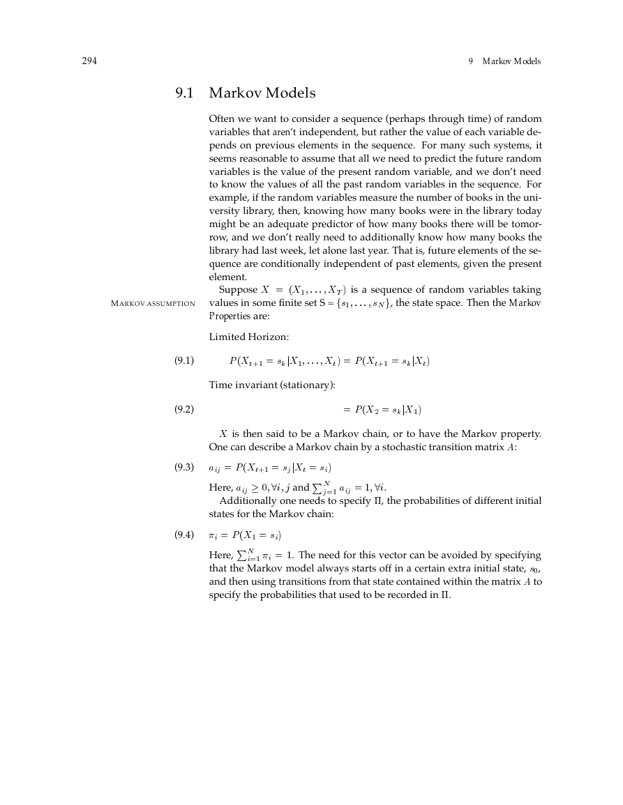
294 9 Markov Models 9.1 Markov Models Often we want to consider a sequence (perhaps through time) of random variables that aren’t independent, but rather the value of each variable de- pends on previous elements in the sequence. For many such systems, it seems reasonable to assume that all we need to predict the future random variables is the value of the present random variable, and we don’t need to know the values of all the past random variables in the sequence. For example, if the random variables measure the number of books in the uni- versity library, then, knowing how many books were in the library today might be an adequate predictor of how many books there will be tomor- row, and we don’t really need to additionally know how many books the library had last week, let alone last year. That is, future elements of the se- quence are conditionally independent of past elements, given the present element. Suppose X X XT is a sequence of random variables taking values in some ﬁnite set S = fs sN g, the state space. Then the Markov Properties are: MARKOV ASSUMPTION Limited Horizon: (9.1) (9.2) P Xt skjX Xt P Xt skjXt Time invariant (stationary): P X skjX X is then said to be a Markov chain, or to have the Markov property. One can describe a Markov chain by a stochastic transition matrix A: (9.3) aij P Xt sjjXt si Here, aij i j and PN Additionally one needs to specify , the probabilities of different initial states for the Markov chain: j aij i. (9.4) i P X si Here, PN i i . The need for this vector can be avoided by specifying that the Markov model always starts off in a certain extra initial state, s, and then using transitions from that state contained within the matrix A to specify the probabilities that used to be recorded in .

9.1 Markov Models 295 h e a t start p i Figure 9.1 A Markov model. From this general description, it should be clear that the word n-gram models we saw in Chapter 6 are Markov models. Markov models can be used whenever one wants to model the probability of a linear sequence of events. For example, they have also been used in NLP for modeling valid phone sequences in speech recognition, and for sequences of speech acts in dialog systems. Alternatively, one can represent a Markov chain by a state diagram as in Figure 9.1. Here, the states are shown as circles around the state name, and the single start state is indicated with an incoming arrow. Possible transitions are shown by arrows connecting states, and these arcs are la- beled with the probability of this transition being followed, given that you are in the state at the tail of the arrow. Transitions with zero probability are omitted from the diagram. Note that the probabilities of the outgoing arcs from each state sum to 1. From this representation, it should be clear that a Markov model can be thought of as a (nondeterministic) ﬁnite state automaton with probabilities attached to each arc. The Markov properties ensure that we have a ﬁnite state automaton. There are no long distance dependencies, and where one ends up next depends simply on what state one is in. In a visible Markov model, we know what states the machine is passing through, so the state sequence or some deterministic function of it can be regarded as the output. The probability of a sequence of states (that is, a sequence of random

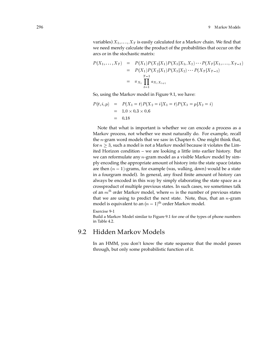
296 9 Markov Models variables) X XT is easily calculated for a Markov chain. We ﬁnd that we need merely calculate the product of the probabilities that occur on the arcs or in the stochastic matrix: P X XT P XP XjXP XjX X P XT jX XT P XP XjXP XjX P XT jXT X T Y t aXtXt So, using the Markov model in Figure 9.1, we have: P t i p P X tP X ijX tP X pjX i Note that what is important is whether we can encode a process as a Markov process, not whether we most naturally do. For example, recall the n-gram word models that we saw in Chapter 6. One might think that, for n , such a model is not a Markov model because it violates the Lim- ited Horizon condition – we are looking a little into earlier history. But we can reformulate any n-gram model as a visible Markov model by sim- ply encoding the appropriate amount of history into the state space (states are then n -grams, for example (was, walking, down) would be a state in a fourgram model). In general, any ﬁxed ﬁnite amount of history can always be encoded in this way by simply elaborating the state space as a crossproduct of multiple previous states. In such cases, we sometimes talk of an mth order Markov model, where m is the number of previous states that we are using to predict the next state. Note, thus, that an n-gram model is equivalent to an n th order Markov model. Exercise 9-1 Build a Markov Model similar to Figure 9.1 for one of the types of phone numbers in Table 4.2. 9.2 Hidden Markov Models In an HMM, you don’t know the state sequence that the model passes through, but only some probabilistic function of it.

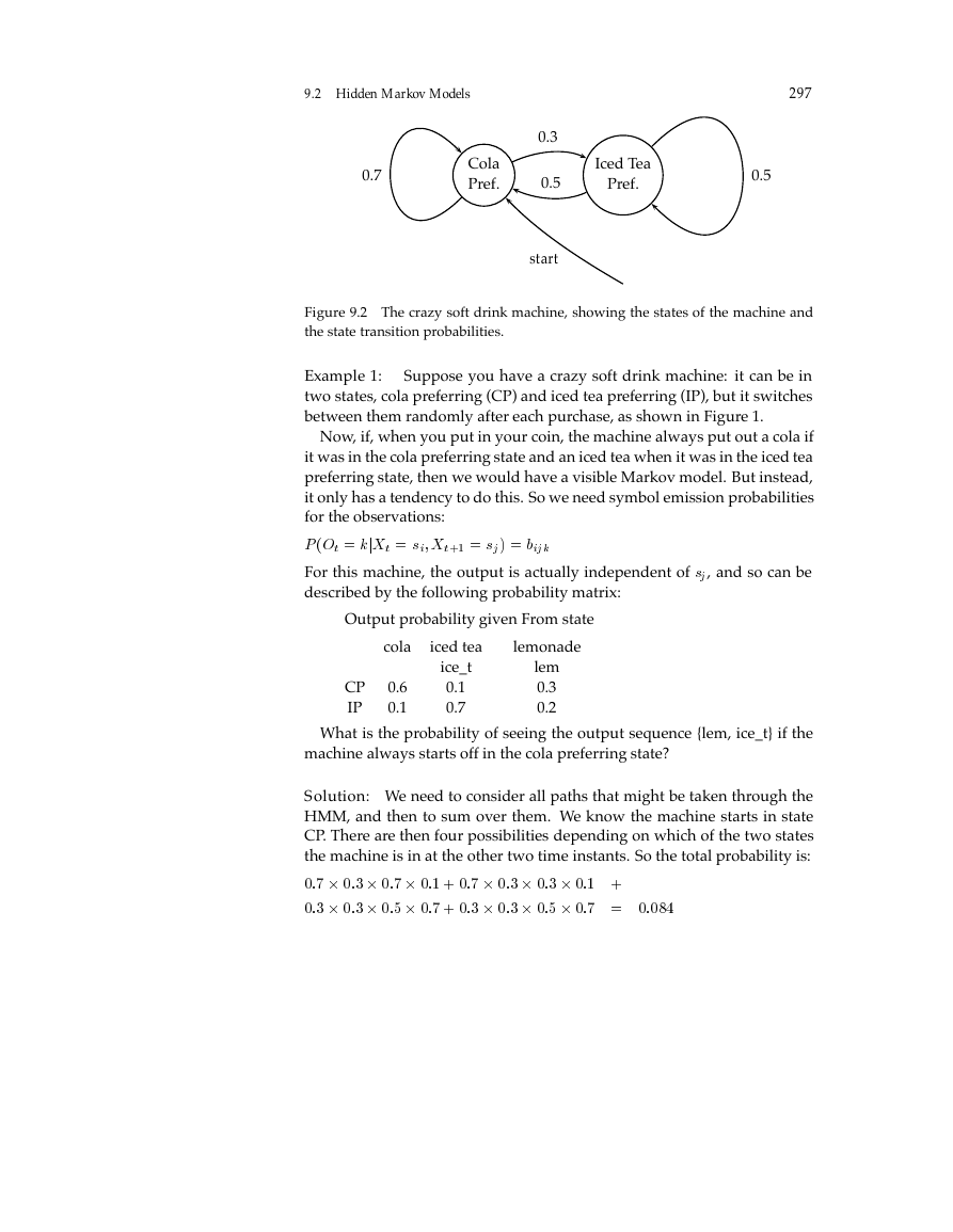
9.2 Hidden Markov Models 297 0.7 Cola Pref. 0.3 0.5 start Iced Tea Pref. 0.5 Figure 9.2 The crazy soft drink machine, showing the states of the machine and the state transition probabilities. Suppose you have a crazy soft drink machine: it can be in Example 1: two states, cola preferring (CP) and iced tea preferring (IP), but it switches between them randomly after each purchase, as shown in Figure 1. Now, if, when you put in your coin, the machine always put out a cola if it was in the cola preferring state and an iced tea when it was in the iced tea preferring state, then we would have a visible Markov model. But instead, it only has a tendency to do this. 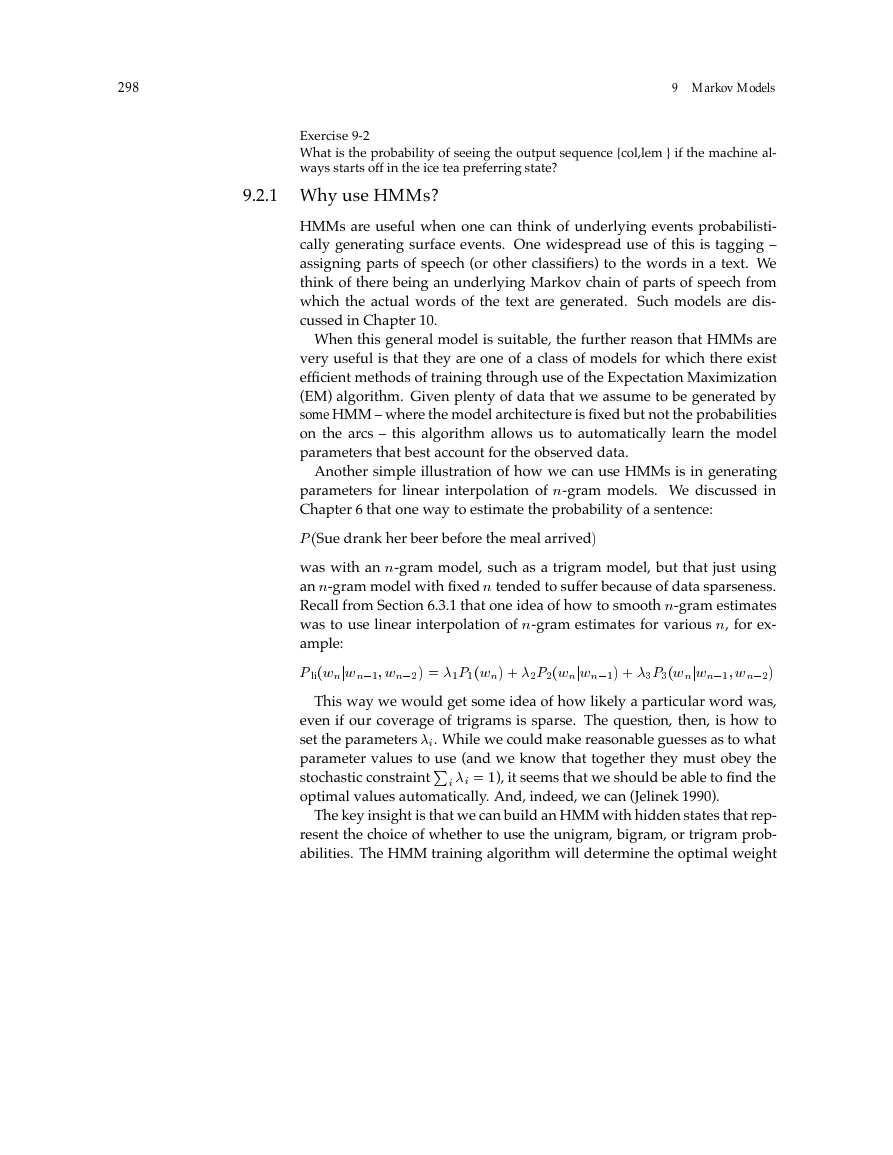So we need symbol emission probabilities for the observations: P Ot kjXt si Xt sj bijk For this machine, the output is actually independent of sj, and so can be described by the following probability matrix: Output probability given From state cola iced tea lemonade CP IP 0.6 0.1 ice_t 0.1 0.7 lem 0.3 0.2 What is the probability of seeing the output sequence {lem, ice_t} if the machine always starts off in the cola preferring state? Solution: We need to consider all paths that might be taken through the HMM, and then to sum over them. We know the machine starts in state CP. There are then four possibilities depending on which of the two states the machine is in at the other two time instants. So the total probability is:

298 9 Markov Models Exercise 9-2 What is the probability of seeing the output sequence {col,lem } if the machine al- ways starts off in the ice tea preferring state? 9.2.1 Why use HMMs? HMMs are useful when one can think of underlying events probabilisti- cally generating surface events. One widespread use of this is tagging – assigning parts of speech (or other classiﬁers) to the words in a text. We think of there being an underlying Markov chain of parts of speech from which the actual words of the text are generated. Such models are dis- cussed in Chapter 10. When this general model is suitable, the further reason that HMMs are very useful is that they are one of a class of models for which there exist efﬁcient methods of training through use of the Expectation Maximization (EM) algorithm. Given plenty of data that we assume to be generated by some HMM – where the model architecture is ﬁxed but not the probabilities on the arcs – this algorithm allows us to automatically learn the model parameters that best account for the observed data. Another simple illustration of how we can use HMMs is in generating parameters for linear interpolation of n-gram models. We discussed in Chapter 6 that one way to estimate the probability of a sentence: P Sue drank her beer before the meal arrived was with an n-gram model, such as a trigram model, but that just using an n-gram model with ﬁxed n tended to suffer because of data sparseness. Recall from Section 6.3.1 that one idea of how to smooth n-gram estimates was to use linear interpolation of n-gram estimates for various n, for ex- ample: P liwnjwn wn Pwn Pwnjwn Pwnjwn wn This way we would get some idea of how likely a particular word was, even if our coverage of trigrams is sparse. The question, then, is how to set the parameters i. While we could make reasonable guesses as to what parameter values to use (and we know that together they must obey the stochastic constraintPi i ), it seems that we should be able to ﬁnd the optimal values automatically. And, indeed, we can (Jelinek 1990). The key insight is that we can build an HMM with hidden states that rep- resent the choice of whether to use the unigram, bigram, or trigram prob- abilities. The HMM training algorithm will determine the optimal weight

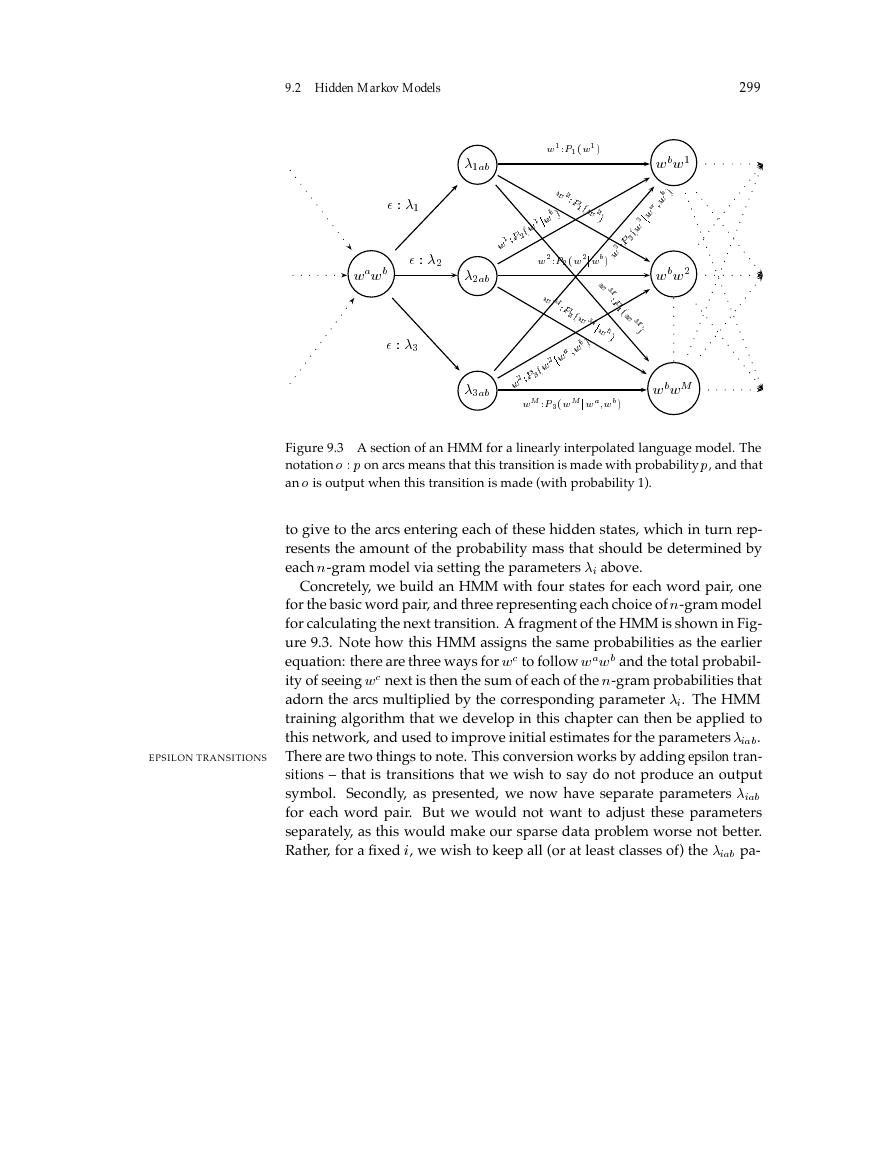
9.2 Hidden Markov Models 299 wPw ab wawb ab w P w b j w w wPwjwb w P w P w wbw b a w jw wbw w M P wM P wM w jwb b w a j w w P w wM PwM jwawb ab M wbwM Figure 9.3 A section of an HMM for a linearly interpolated language model. The notation o p on arcs means that this transition is made with probability p, and that an o is output when this transition is made (with probability 1). to give to the arcs entering each of these hidden states, which in turn rep- resents the amount of the probability mass that should be determined by each n-gram model via setting the parameters i above. Concretely, we build an HMM with four states for each word pair, one for the basic word pair, and three representing each choice of n-gram model for calculating the next transition. A fragment of the HMM is shown in Fig- ure 9.3. Note how this HMM assigns the same probabilities as the earlier equation: there are three ways for wc to follow wawb and the total probabil- ity of seeing wc next is then the sum of each of the n-gram probabilities that adorn the arcs multiplied by the corresponding parameter i. The HMM training algorithm that we develop in this chapter can then be applied to this network, and used to improve initial estimates for the parameters iab. There are two things to note. This conversion works by adding epsilon tran- sitions – that is transitions that we wish to say do not produce an output symbol. Secondly, as presented, we now have separate parameters iab for each word pair. But we would not want to adjust these parameters separately, as this would make our sparse data problem worse not better. Rather, for a ﬁxed i, we wish to keep all (or at least classes of) the iab pa- EPSILON TRANSITIONS

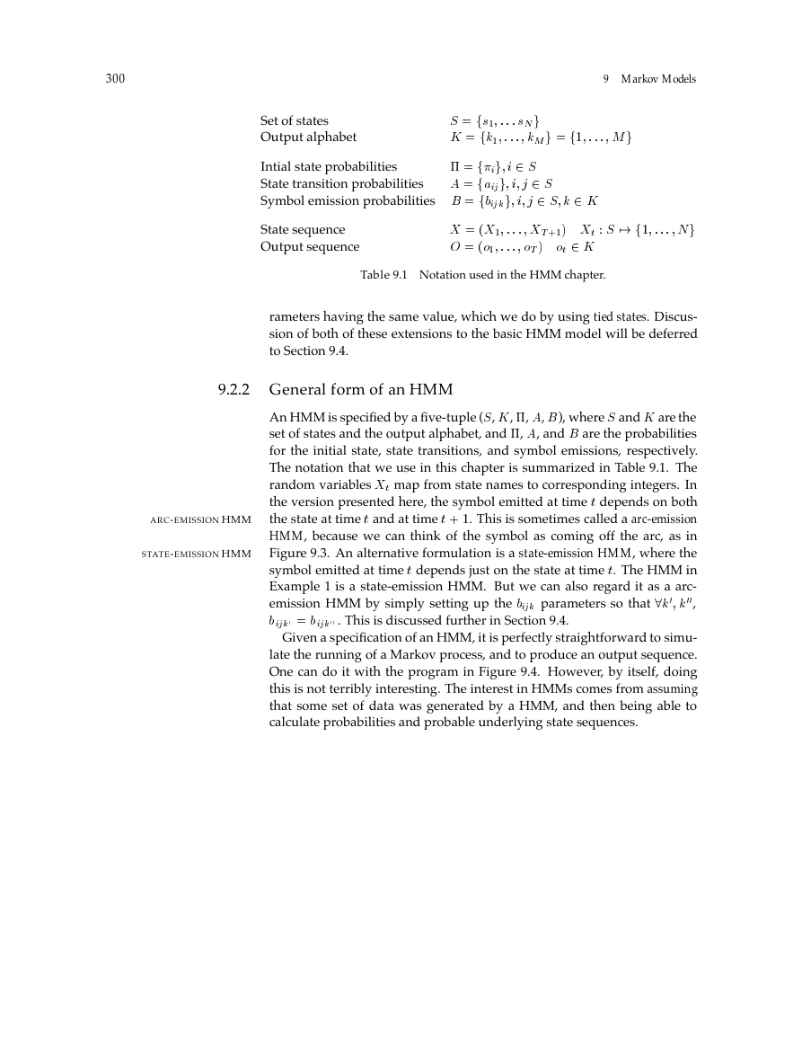
300 9 Markov Models Set of states Output alphabet S fs sN g K fk kM g f M g Intial state probabilities State transition probabilities Symbol emission probabilities B fbijkg i j S k K fig i S A faijg i j S State sequence Output sequence X X XT Xt S f N g O o oT ot K Table 9.1 Notation used in the HMM chapter. rameters having the same value, which we do by using tied states. Discus- sion of both of these extensions to the basic HMM model will be deferred to Section 9.4. 9.2.2 General form of an HMM ARC-EMISSION HMM STATE-EMISSION HMM An HMM is speciﬁed by a ﬁve-tuple (S, K, , A, B), where S and K are the set of states and the output alphabet, and , A, and B are the probabilities for the initial state, state transitions, and symbol emissions, respectively. The notation that we use in this chapter is summarized in Table 9.1. The random variables Xt map from state names to corresponding integers. In the version presented here, the symbol emitted at time t depends on both the state at time t and at time t . This is sometimes called a arc-emission HMM, because we can think of the symbol as coming off the arc, as in Figure 9.3. An alternative formulation is a state-emission HMM, where the symbol emitted at time t depends just on the state at time t. The HMM in Example 1 is a state-emission HMM. But we can also regard it as a arc- emission HMM by simply setting up the bijk parameters so that k k, bijk bijk . This is discussed further in Section 9.4. Given a speciﬁcation of an HMM, it is perfectly straightforward to simu- late the running of a Markov process, and to produce an output sequence. One can do it with the program in Figure 9.4. However, by itself, doing this is not terribly interesting. The interest in HMMs comes from assuming that some set of data was generated by a HMM, and then being able to calculate probabilities and probable underlying state sequences.

分享到：

赞收藏

资料库

Markov Models（马尔可夫模型讲解）.pdf

相关推荐

开发技术

热门标签

最新资料